ALSSM Trajectory [code102.0]¶

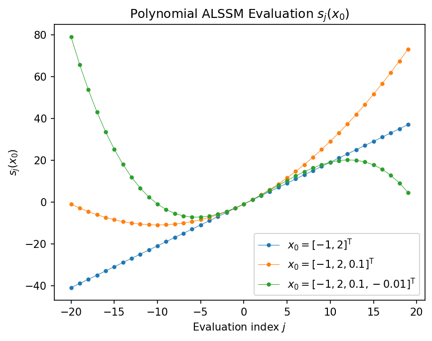
Evaluates an ALSSM over a time range for a given initial state vector.

eval_output computes the output sequence \(s_j(x_0) = C A^j x_0\) for a range of evaluation indices \(j\). Three polynomial ALSSMs of degree 1, 2, and 3 are evaluated and plotted together.

Plot¶

Plot

Console Output¶

--DUMP--
 └-AlssmPoly, A: (4, 4), C: (4,), label: 3rd degree
--PRINT--
 AlssmPoly(A=[[1 1 1 1] [0 1 2 3] [0 0 1 3] [0 0 0 1]], C=[1 0 0 0], label=3rd degree)

Code¶

"""
ALSSM Trajectory [code102.0]
==========================

Evaluates an ALSSM over a time range for a given initial state vector.

[`eval_output`][lmlib.statespace.model.ModelBase.eval_output] computes the output
sequence $s_j(x_0) = C A^j x_0$ for a range of evaluation indices
$j$.  Three polynomial ALSSMs of degree 1, 2, and 3 are evaluated and
plotted together.

See also:
[`eval_output`][lmlib.statespace.model.ModelBase.eval_output]

"""

import matplotlib.pyplot as plt
import lmlib as lm


js = range(-20, 20)  # ALSSM evaluation range

alssm = lm.AlssmPoly(poly_degree=1, label='1th degree')
x0_d1 = [-1, 2]  # initial state vector
sx0_d1 = alssm.eval_output(x0_d1, js)

alssm = lm.AlssmPoly(poly_degree=2, label='2nd degree')
x0_d2 = [-1, 2, .1]  # initial state vector
sx0_d2 = alssm.eval_output(x0_d2, js)

alssm = lm.AlssmPoly(poly_degree=3, label='3rd degree')
x0_d3 = [-1, 2, .1, -.01]  # initial state vector
sx0_d3 = alssm.eval_output(x0_d3, js)

# Printing Model to Console
print("--DUMP--\n", alssm.dump_tree())
print("--PRINT--\n", alssm)

# plot
plt.plot(js, sx0_d1, '.-', lw=.5, label=r'$x_0 = ' + str(x0_d1) + r'^\mathrm{T}$')
plt.plot(js, sx0_d2, '.-', lw=.5, label=r'$x_0 = ' + str(x0_d2) + r'^\mathrm{T}$')
plt.plot(js, sx0_d3, '.-', lw=.5, label=r'$x_0 = ' + str(x0_d3) + r'^\mathrm{T}$')
plt.xlabel('Evaluation index $j$')
plt.ylabel('$s_j(x_0)$')
plt.title('Polynomial ALSSM Evaluation $s_j(x_0)$')
plt.legend()
plt.show()