Single-Segment (CostSegment) Models: Trajectories and Windows [code103.0]¶

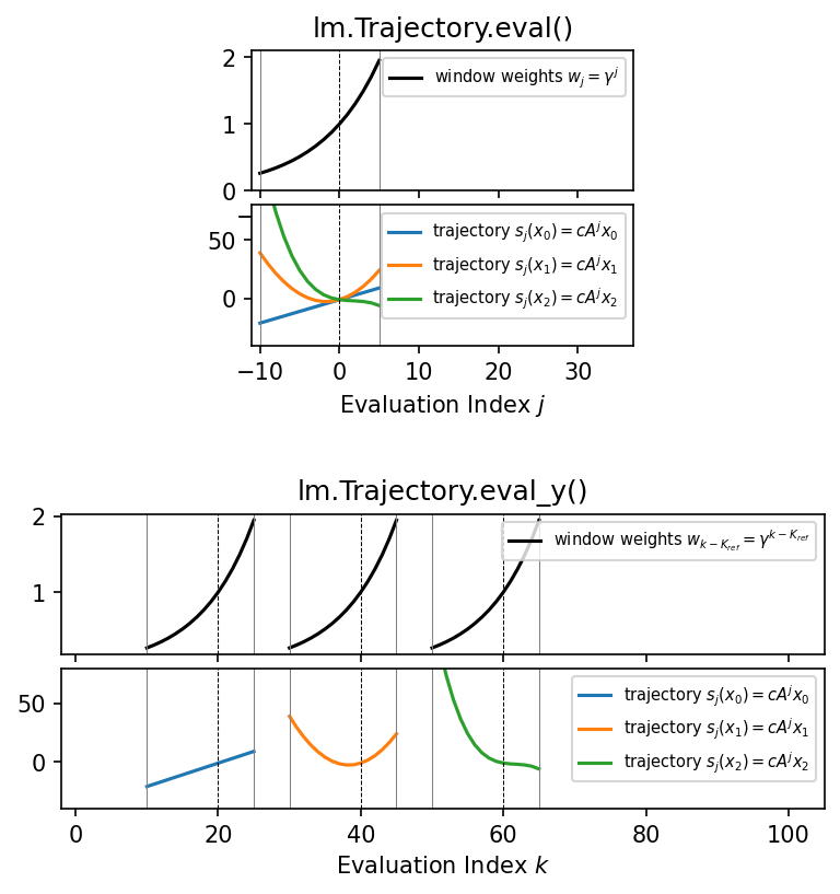
Defines a cost segment consisting of an ALSSM and a left-sided, exponentially decaying window, then visualises the window weights and the resulting signal trajectories for a set of state vectors.

Two plot groups are shown:

Upper plots — the window and trajectories in the relative index domain (centred at \(j=0\)).
Lower plots — the same trajectories placed at absolute signal positions K_refs in a length-K output vector.

Plot¶

Plot

Console Output¶

-- Print --
CostSegment(label: costs segment for polynomial model) 
  └- AlssmPoly(A=[[1 1 1 1] [0 1 2 3] [0 0 1 3] [0 0 0 1]], C=[1 0 0 0], label=alssm-polynomial), 
  └- Segment(a=-10, b=5, direction=fw, g=8, delta=0, label=left-decaying)

/home/runner/work/lmlib/lmlib/coding/10-windowed-state-space-filters-basic/_temp_coding-code103.0-cost-segment.py:134: UserWarning: No artists with labels found to put in legend.  Note that artists whose label start with an underscore are ignored when legend() is called with no argument.
  ax.legend(fontsize=7, loc=1)

Code¶

"""
Single-Segment (CostSegment) Models: Trajectories and Windows [code103.0]
=======================================================================

Defines a cost segment consisting of an ALSSM and a left-sided,
exponentially decaying window, then visualises the window weights and
the resulting signal trajectories for a set of state vectors.

Two plot groups are shown:

* **Upper plots** — the window and trajectories in the relative index
  domain (centred at $j=0$).
* **Lower plots** — the same trajectories placed at absolute signal
  positions ``K_refs`` in a length-``K`` output vector.

See also:
[`CostSegment`][lmlib.statespace.cost.CostSegment],
[`Segment`][lmlib.statespace.segment.Segment]
"""
import matplotlib.pyplot as plt
import lmlib as lm
import numpy as np

# Defining a second order polynomial ALSSM
alssm_poly = lm.AlssmPoly(poly_degree=3, label="alssm-polynomial")

# Defining a segment with a left-sided, exponentially decaying window
a = -10  # left boundary
b = 5  # right boundary
g = 8  # effective number of weighted samples under the window (controls window size)
left_seg = lm.Segment(a, b, lm.FORWARD, g, label="left-decaying")

# creating the cost segment, combining window (segment) and model (ALSSM).
costs = lm.CostSegment(alssm_poly, left_seg, label="costs segment for polynomial model")

# print internal structure
print('-- Print --')
print(costs)

# get trajectory from initial state
xs = np.array([[-1, 2, 0, 0],  # polynomial coefficients of trajectories
      [-1, 2, .6, 0],
      [-1, -1, .4, -.08]])

# --------- Upper Plots ---------
# get window weights

# Window
windows = lm.Window.eval(costs)
js, w = windows[0]

# Trajectories
trajectories = lm.Trajectory.eval(costs, xs, merged_ks=False)

# plot
fig, axs = plt.subplots(5, gridspec_kw={'hspace': 0.1}, figsize=(6, 6))

# Shrink top two axes horizontally and center them
for ax in [axs[0], axs[1]]:
    pos = ax.get_position()
    new_width = pos.width * 0.5      # keep 60% of original width
    new_x0 = pos.x0 + (pos.width - new_width) / 2
    ax.set_position([new_x0, pos.y0, new_width, pos.height])

axs[0].plot(js,w, '-', c='k', lw=1.5, label=r'window weights $w_j = \gamma^j$')
axs[0].set_title('lm.Trajectory.eval()')
axs[0].axvline(0, color="black", linestyle="--", lw=0.5)
axs[0].axvline(a, color="gray", linestyle="-", lw=0.5)
axs[0].axvline(b, color="gray", linestyle="-", lw=0.5)
axs[0].set(ylim=[0, 2.1])
axs[0].set(xlim=[-11, 37])

for n, trajectory_p in enumerate(trajectories):
    js, trajectory = trajectory_p
    axs[1].plot(js, trajectory, lw=1.5, label=r'trajectory $s_j(x_' + str(n) + ') = cA^jx_' + str(n) + '$')

# ideas for alternative plotting functions:
# ax = traj_obj.plot_merged(axs[1], lw=1.5, label='trajectory $s_j$')
# ax = traj_obj.plot_merged_segments(axs[1], lw=1.5, label=['trajectory $s_j$' for ..])
# ax = traj_obj.plot_merged_states(axs[1], lw=1.5, label=['trajectory $s_j$' for ..])

axs[1].set_xlabel('Evaluation Index $j$')
axs[1].axvline(0, color="black", linestyle="--", lw=0.5)
axs[1].axvline(a, color="gray", linestyle="-", lw=0.5)
axs[1].axvline(b, color="gray", linestyle="-", lw=0.5)
axs[1].set(ylim=[-40, 80])
axs[1].set(xlim=[-11, 37])

axs[1].tick_params(axis='both', which='both', labelbottom=True)

axs[2].set_visible(False)  # add spacer

# --------- Lower Plots ---------
# Get localized trajectories
K = 70  # total signal length
K_refs = [20, 40, 60]  # trajectory locations (indices)
COLS_W = ['black', 'gray', 'lightgray']

windows = lm.Window.eval_y(costs, K_refs, K, merged_seg=True,fill_value=np.nan)
axs[3].plot(windows, c='k', lw=1.5, label=r"window weights $w_{k-K_{ref}}=\gamma^{k-K_{ref}}$")
axs[3].set(xlim=[-2, 105])
axs[3].set_title('lm.Trajectory.eval_y()')

trajectories = lm.Trajectory.eval_y(costs, xs, K_refs, K, merged_ks=False)
#axs[4].plot(trajectories, lw=2, label='y_hat')
for n, trajectory_p in enumerate(trajectories):
    axs[4].plot(trajectory_p, lw=1.5, label=r'trajectory $s_j(x_' + str(n) + ') = cA^jx_' + str(n) + '$')


for k_ref in K_refs:
    axs[3].axvline(k_ref + a, color="gray", linestyle="-", lw=0.5)
    axs[3].axvline(k_ref + b, color="gray", linestyle="-", lw=0.5)
    axs[3].axvline(k_ref, color="black", linestyle="--", lw=0.5)
    axs[4].axvline(k_ref + a, color="gray", linestyle="-", lw=0.5)
    axs[4].axvline(k_ref + b, color="gray", linestyle="-", lw=0.5)
    axs[4].axvline(k_ref, color="black", linestyle="--", lw=0.5)

axs[4].set_xlabel('Evaluation Index $k$')
axs[4].set(ylim=[-40, 80])
axs[4].set(xlim=[-2, 105])

for ax in axs:
    ax.legend(fontsize=7, loc=1)
plt.show()