Composed ALSSM Windows (Weighting Window) [code104.0]
Each cost segment in lmlib.statespace.cost is weighted by its own
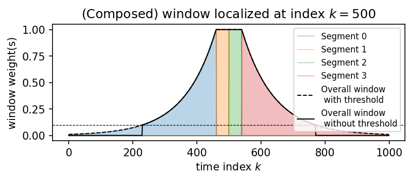
exponential window function. This guide script demonstrates the basic
exponentially decaying window of both finite and infinite support, and shows
how a more complex symmetric window is built by composing four such segments.
The composed window consists of two exponentially decaying tails (left and
right) and a near-rectangular centre region, all joined into a single
CompositeCost.
Plot
Code
"""
Composed ALSSM Windows (Weighting Window) [code104.0]
===================================================

Each cost segment in [`lmlib.statespace.cost`][lmlib.statespace.cost] is weighted by its own
exponential window function.  This guide script demonstrates the basic
exponentially decaying window of both finite and infinite support, and shows
how a more complex symmetric window is built by composing four such segments.

The composed window consists of two exponentially decaying tails (left and
right) and a near-rectangular centre region, all joined into a single
[`CompositeCost`][lmlib.statespace.cost.CompositeCost].

See also:
[`window`][lmlib.statespace.segment.Segment.window],
[`Window`][lmlib.statespace.window.Window]

"""

import numpy as np
import matplotlib.pyplot as plt
import lmlib as lm

K = 1000  # signal length
ks = 500  # (arbitrary) window location
k = range(K)

segment_left_infinite = lm.Segment(a=-np.inf, b=-40, direction=lm.FORWARD, g=100, delta=-40)  # left decaying window
segment_left_finite = lm.Segment(a=-39, b=-1, direction=lm.FORWARD, g=1e6, delta=0)  # (nearly) rectangular window
segment_right_finite = lm.Segment(a=0, b=39, direction=lm.BACKWARD, g=1e6, delta=0)  # (nearly) rectangular window
segment_right_infinite = lm.Segment(a=40, b=np.inf, direction=lm.BACKWARD, g=100, delta=40)  # right decaying window

cost = lm.CompositeCost((lm.AlssmPoly(3),),
                        [segment_left_infinite, segment_left_finite, segment_right_finite, segment_right_infinite],
                        F=[[1, 1, 1, 1]])

# Generating Windows - for illustrative and plotting purposes only
# ---------------------------------------------------------------

# Minimum window weight below which samples are treated as zero.
# Only relevant for exponentially decaying windows with infinite support,
# which never reach exactly 0.
display_thd = 0.1
# Per-segment windows without thresholding
wins = lm.Window.eval_y(cost, ks, K, merged_seg=False)

# Combined window with thresholding applied (infinite tails clipped at display_thd)
wins_all_no_thd = lm.Window.eval_y(cost, ks, K, merged_seg=True,thd=display_thd)
# Combined window without thresholding (infinite tails shown in full)
wins_all = lm.Window.eval_y(cost, ks, K, merged_seg=True)

# Plot
# ----
plt.figure(figsize=(6, 2))
for p, win in enumerate(wins):
    line = plt.plot(k, win, '-', lw=0.3, label=f'Segment {p}')
    plt.fill_between(k, win, color=line[0].get_color(), alpha=0.3)
plt.plot(k, wins_all, '--k', lw=1.0, label='Overall window \n with threshold')
plt.plot(k, wins_all_no_thd, '-k', lw=1.0, label='Overall window \n without threshold')

plt.axhline(display_thd, lw=0.6, c='k', ls='--', label='')
plt.xlabel('time index $k$')
plt.ylabel('window weight(s)')
plt.title(f'(Composed) window localized at index $k={ks}$')
plt.legend(loc=1, fontsize=8)
plt.show()