Multi-Segment (Composite) Models: Windows and Trajectories [code105.0]

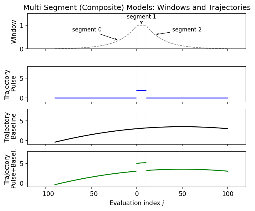
Defines a CompositeCost combining two ALSSM models (a pulse model and a baseline model) with three segments (left, centre, right), and visualises the resulting windows and trajectories.

The mapping matrix F selects which ALSSM is active in each segment: the pulse model covers only the centre segment, while the baseline model spans all three. Separate trajectory plots are shown for the pulse-only, baseline-only, and combined (pulse + baseline) contributions.

Plot

Code

"""
Multi-Segment (Composite) Models: Windows and Trajectories [code105.0]
====================================================================

Defines a [`CompositeCost`][lmlib.statespace.cost.CompositeCost] combining two ALSSM
models (a pulse model and a baseline model) with three segments (left, centre,
right), and visualises the resulting windows and trajectories.

The mapping matrix ``F`` selects which ALSSM is active in each segment:
the pulse model covers only the centre segment, while the baseline model
spans all three.  Separate trajectory plots are shown for the pulse-only,
baseline-only, and combined (pulse + baseline) contributions.

"""
import matplotlib.pyplot as plt
import numpy as np
from scipy.signal import find_peaks

import lmlib as lm
from lmlib.utils.generator import (gen_rand_pulse, gen_wgn, gen_rand_walk)


# Defining ALSSM models
alssm_pulse = lm.AlssmPoly(poly_degree=0, label="line-model-pulse")
alssm_baseline = lm.AlssmPoly(poly_degree=2, label="offset-model-baseline")

# Defining segments with a left- resp. right-sided decaying window and a center segment with a nearly rectangular window
segment_left = lm.Segment(a=-np.inf, b=-1, direction=lm.FORWARD, g=20)
segment_center= lm.Segment(a=0, b=10, direction=lm.FORWARD, g=5000)
segment_right = lm.Segment(a=10+1, b=np.inf, direction=lm.BACKWARD, g=20, delta=10)

# Defining the final cost function
# mapping matrix between models and segments (rows = models, columns = segments)
F = [[0, 1, 0],
     [1, 1, 1]]

costs = lm.CompositeCost((alssm_pulse, alssm_baseline), (segment_left, segment_center, segment_right), F)
x0 = [2, 3, 0.02, -0.0002] # initial states of alssm_pulse [0:1] and of alssm_baseline [1:4]

windows = lm.Window.eval(costs,thd=0.01)


F_baseline_only = [[0, 0, 0],
                   [1, 1, 1]]
F_pulse_only    = [[0, 1, 0],
                   [0, 0, 0]]

# Trajectories
trajectories_baseline = lm.Trajectory.eval(costs, x0, F_baseline_only, thd=0.01,merged_seg=False)
trajectories_pulse = lm.Trajectory.eval(costs,x0, F_pulse_only, thd=0.01,merged_seg=False)
trajectories = lm.Trajectory.eval(costs,x0, F, thd=0.01,merged_seg=False)

fig, axs = plt.subplots(4, sharex='all')

# Plot Window — same colour and linestyle for all three segments; the segments
# are annotated directly in the plot (no legend).
for (js, weights), loc in zip(windows, ('0', '1', '2')):
    axs[0].plot(js, weights, c='gray', ls='--', lw=1.0)
axs[0].set_ylabel('Window')
axs[0].set_ylim([-0, 1.5])

# In-plot annotation of the three segments (arrow -> a point on each lobe).
seg_labels  = ('segment 0', 'segment 1', 'segment 2')
seg_arrow_x = (-20, 5, 20)
seg_text_xy = ((-55, 0.75), (5, 1.30), (55, 0.75))
for (js, weights), name, ax_x, txy in zip(windows, seg_labels, seg_arrow_x, seg_text_xy):
    js = np.asarray(js); weights = np.asarray(weights)
    order = np.argsort(js)
    y_on_curve = float(np.interp(ax_x, js[order], weights[order]))
    axs[0].annotate(name, xy=(ax_x, y_on_curve), xytext=txy, ha='center',
                    fontsize=9, color='black',
                    arrowprops=dict(arrowstyle='->', lw=0.8, color='black'))

# Trajectory subplots: one colour per *signal* (not per segment) — pulse=blue,
# baseline=black, pulse+baseline=green; all three segments share that colour.
# Plot Trajectory Pulse (blue)
for (js, trajs), loc in zip(trajectories_pulse, ('0', '1', '2')):
    axs[1].plot(js, trajs, lw=1.5, c='blue')
axs[1].set_ylabel('Trajectory\n Pulse')
axs[1].set_ylim([-1, 8.0])

# Plot Trajectory Baseline (black)
for (js, trajs), loc in zip(trajectories_baseline, ('0', '1', '2')):
    axs[2].plot(js, trajs, lw=1.5, c='black')
axs[2].set_ylabel('Trajectory\n Baseline')
axs[2].set_ylim([-1, 8.0])

# Plot Trajectory Pulse+Baseline (green)
for (js, trajs), loc in zip(trajectories, ('0', '1', '2')):
    axs[3].plot(js, trajs, lw=1.5, c='green')
axs[3].set_ylabel('Trajectory\n Pulse+Basel.')
axs[3].set_ylim([-1, 8.0])

axs[-1].set_xlabel('Evaluation index $j$')
axs[0].set_title('Multi-Segment (Composite) Models: Windows and Trajectories')
axs[0].set_xlim([-120, 120])

for _ax in axs:
    _ax.axvline(0,  color="black", linestyle="--", lw=0.5)
    _ax.axvline(10, color="black", linestyle="--", lw=0.5)

# Add a bit of extra spacing between the window subplot (0) and the trajectory
# subplots (1-3) by nudging the top axes upward.
fig.canvas.draw()
pos0 = axs[0].get_position()
axs[0].set_position([pos0.x0, pos0.y0 + 0.05, pos0.width, pos0.height])

plt.show()