Local Signal Approximation with Increasing Polynomial Degree [code106.0]

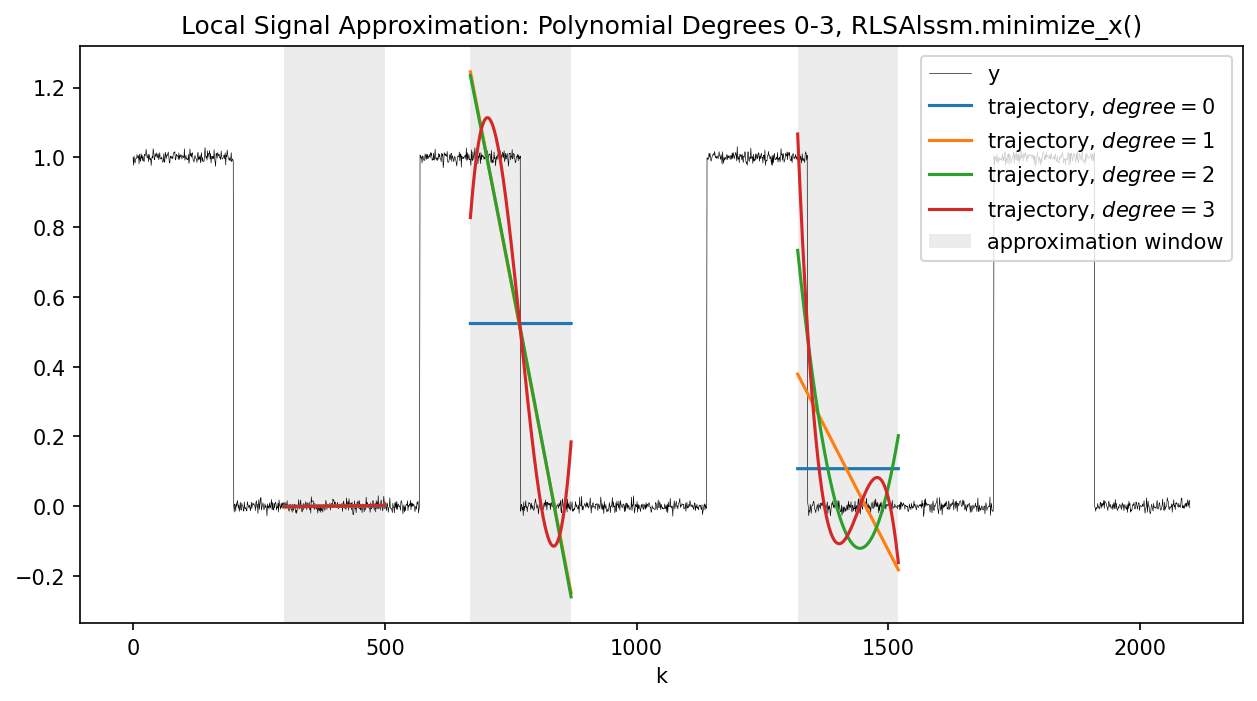
Fits local polynomial models of increasing degree to a rectangular test signal using RLSAlssm with the Pascal monomial basis (AlssmPoly), in the spirit of the multi-degree filter sweep in example-ex122.0-polynomial-filters.py.

For each degree, the optimal state vector is extracted at three reference positions and the corresponding trajectory is placed at the correct absolute location in the output signal. Only well-conditioned approximations are shown: the Pascal basis is swept up to degree 4 only, beyond which it becomes numerically ill-conditioned for this window length (higher degrees would need a numerically superior basis such as Legendre).

Plot

Code

"""
Local Signal Approximation with Increasing Polynomial Degree [code106.0]
=======================================================================

Fits local polynomial models of increasing degree to a rectangular test signal
using [`RLSAlssm`][lmlib.statespace.rls.RLSAlssm] with the Pascal monomial basis
([`AlssmPoly`][lmlib.statespace.model.AlssmPoly]), in the spirit of the
multi-degree filter sweep in ``example-ex122.0-polynomial-filters.py``.

For each degree, the optimal state vector is extracted at three reference
positions and the corresponding trajectory is placed at the correct absolute
location in the output signal.  Only well-conditioned approximations are shown:
the Pascal basis is swept up to degree 4 only, beyond which it becomes
numerically ill-conditioned for this window length (higher degrees would need a
numerically superior basis such as Legendre).
"""
import matplotlib.pyplot as plt
import lmlib as lm
from lmlib.utils.generator import gen_wgn, gen_rect

plt.close('all')

K = 2100
y = gen_rect(K, 570, 200) + gen_wgn(K, 0.01)

g = 1000
K_refs = [300, 670, 1320]

# Sweep polynomial degrees. The Pascal (monomial) basis is numerically
# well-conditioned only up to ~degree 4 for this window length, so only those
# (good) approximations are shown.
degrees = [0, 1, 2, 3]
STYLES = ['tab:blue', 'tab:orange', 'tab:green', 'tab:red', 'tab:purple', 'tab:brown']

plt.figure(figsize=(10, 5))
plt.plot(y, lw=0.3, c='k', label='y')

for i, pd in enumerate(degrees):
    cost = lm.CostSegment(lm.AlssmPolyJordan(poly_degree=pd), lm.Segment(0, 200, lm.BW, g))
    rls = lm.RLSAlssm(cost)
    rls.filter(y)
    xs = rls.minimize_x(solver='lstsq')
    trajs = lm.Trajectory.eval_y(cost, xs[K_refs], K_refs, K, thd=0.01, merged_ks=True, merged_seg=True)
    plt.plot(trajs, lw=1.5, c=STYLES[i], label=rf'trajectory, $degree={pd}$')

# Shade each approximation window [k_ref, k_ref+200] so the local fitting region
# of every trajectory is clearly visible (clearer than full-height grid lines).
for n, _k in enumerate(K_refs):
    plt.axvspan(_k, _k + 200, color='gray', alpha=0.15, lw=0,
                label='approximation window' if n == 0 else None)


plt.title('Local Signal Approximation: Polynomial Degrees 0-3, '
          'RLSAlssm.minimize_x()')
#plt.ylim([-3, 3])
plt.legend(loc=1)
plt.xlabel('k')
plt.show()