Alternative ALSSM Outputs [code107.0]
Demonstrates different ways to reconstruct the signal estimate from the
state vectors returned by minimize_x.
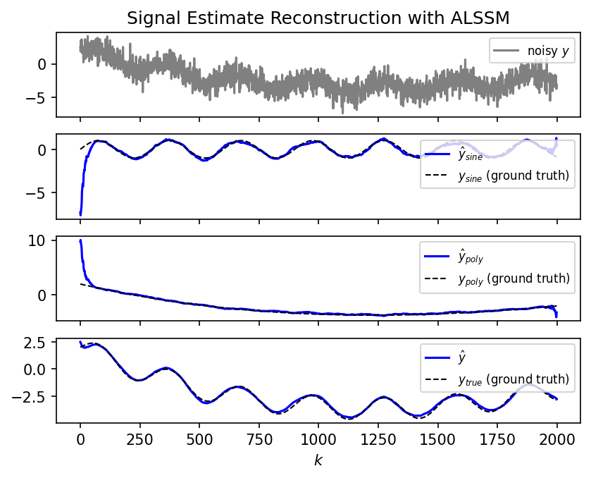
A CompositeCost combines a polynomial and a
sinusoidal ALSSM. After filtering and minimization, two output methods are
compared:
- Normal output — all ALSSMs contribute equally (
alssm_weights=None). - Weighted output — only the sinusoidal component is selected by passing
alssm_weights=(0, 1), setting the polynomial contribution to zero.
Plot
Code
"""
Alternative ALSSM Outputs [code107.0]
===================================

Demonstrates different ways to reconstruct the signal estimate from the
state vectors returned by [`minimize_x`][lmlib.statespace.rls.RLSAlssm.minimize_x].

A [`CompositeCost`][lmlib.statespace.cost.CompositeCost] combines a polynomial and a
sinusoidal ALSSM.  After filtering and minimization, two output methods are
compared:

* **Normal output** — all ALSSMs contribute equally (``alssm_weights=None``).
* **Weighted output** — only the sinusoidal component is selected by passing
  ``alssm_weights=(0, 1)``, setting the polynomial contribution to zero.

"""
import numpy as np
import matplotlib.pyplot as plt
import lmlib as lm
from lmlib.utils import gen_wgn, gen_sine, gen_rand_walk, k_period_to_omega

# create signal
seed = 42
K = 2000
k = np.arange(K)
k_periods = 300
# ground-truth (noise-free) components of the synthetic signal
y_sine = gen_sine(K, k_periods)
# Generate random coefficients for a polynomial
# Strong scaling to prevent explosion
coeffs = np.array([-5e-10, 5e-6, -1e-2, 2])
y_poly = np.polyval(coeffs, k)
#y_poly = 0.05 * gen_rand_walk(K, seed=seed)
ys = y_sine + y_poly + gen_wgn(K, 1, seed=seed)

# create model
alssms = (lm.AlssmPoly(1), lm.AlssmSin(k_period_to_omega(k_periods)))
segments = (lm.Segment(-100, -1, lm.FW, g=100), lm.Segment(0, 99, lm.BW, g=100))
F = np.ones((2, 2))
cost = lm.CompositeCost(alssms, segments, F)

# filter and minimize
rls = lm.RLSAlssm(cost, backend='numpy', steady_state=False)
rls.filter(ys)
xs = rls.minimize_x()

# ------------------------------
# normal output defined by the model
ys_hat_normal = cost.eval_alssm_output(xs)

# ------------------------------
# alternative outputs with alssm weights parameter, Sinusoidal Model only
ys_hat_sinus = cost.eval_alssm_output(xs, alssm_weights=(0, 1))

# alternative outputs with alssm weights parameter, Polynomial Model only
ys_hat_poly = cost.eval_alssm_output(xs, alssm_weights=(1, 0))

fig, axs = plt.subplots(4, sharex='all')

# Ground-truth (noise-free) component matching each estimate, overlaid as a black
y_sine_poly = y_sine + y_poly

# One signal per subplot, each estimate in its own colour (cf. code104): measured
# signal gray, full estimate blue, sinusoidal component green, polynomial component orange.
axs[0].plot(k, ys, c='gray',label=r'noisy $y$')
axs[0].legend(fontsize=8, loc='upper right')

axs[1].plot(k, ys_hat_sinus, lw=1.5, c='b', label=r'$\hat{y}_{sine}$')
axs[1].plot(k, y_sine, c='k', ls='--', lw=1.0, label='${y}_{sine}$ (ground truth)')
axs[1].legend(fontsize=8, loc='upper right')

axs[2].plot(k, ys_hat_poly, lw=1.5, c='b', label=r'$\hat{y}_{poly}$')
axs[2].plot(k, y_poly, c='k', ls='--', lw=1.0, label='${y}_{poly}$ (ground truth)')
axs[2].legend(fontsize=8, loc='upper right')

axs[3].plot(k, ys_hat_normal, lw=1.5, c='b', label=r'$\hat{y}$')
axs[3].plot(k, y_sine_poly, c='k', ls='--', lw=1.0, label='$y_{true}$ (ground truth)')
axs[3].legend(fontsize=8, loc='upper right')


axs[0].set_title('Signal Estimate Reconstruction with ALSSM')
axs[-1].set_xlabel(r'$k$')
plt.show()