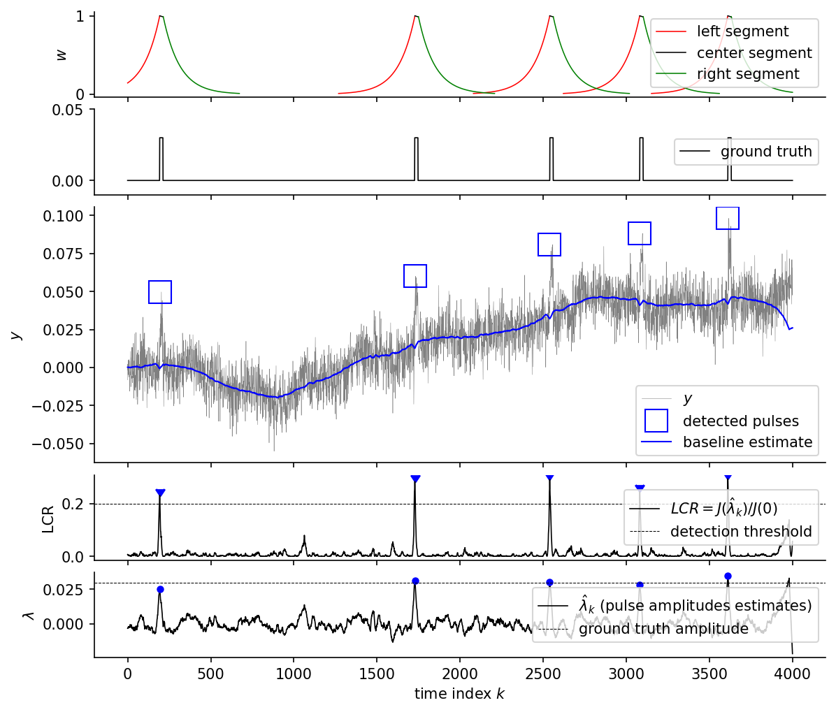
Rectangular Pulse Detection with Baseline [ex111.0]

This example demonstrates the detection of a rectangular pulses of known duration in a noisy signal with baseline interferences.

Plot

Code

# -*- coding: utf-8 -*-
# Author: Waldmann Frédéric, Wildhaber Reto
r"""
Rectangular Pulse Detection with Baseline [ex111.0]
===================================================

This example demonstrates the detection of a rectangular pulses of known duration in a noisy signal with baseline
interferences.

"""
import matplotlib.pyplot as plt
import numpy as np
from lmlib.utils.generator import gen_rand_pulse, gen_wgn, gen_rand_walk
from scipy.signal import find_peaks

import lmlib as lm

# --------------- parameters of example -----------------------
K = 4000  # number of samples (length of test signal)
k = np.arange(K)
len_pulse = 20  # [samples] number of samples of the pulse width
amplitude_pulse = 0.03
y_rpulse = amplitude_pulse*gen_rand_pulse(K, n_pulses=5, length=len_pulse, seed=1010)
y = y_rpulse + gen_wgn(K, sigma=0.01, seed=1000) + 1e-3*gen_rand_walk(K,seed=1001)

LCR_THD = 0.2  # minimum log-cost ratio to detect a pulse in noise

g_sp = 1500  # pulse window weight, effective sample number under the window # (larger value lead to a more rectangular-like windows while too large values might lead to nummerical instabilities in the recursive computations.)
g_bl = 100  # baseline window weight, effective sample number under the window (larger value leads to a wider window)

# --------------- main -----------------------

# Defining ALSSM models
alssm_pulse = lm.AlssmPolyJordan(poly_degree=0, label="line-model-pulse")
alssm_baseline = lm.AlssmPolyJordan(poly_degree=2, label="offset-model-baseline")

# Defining segments with a left-resp. right-sided decaying window and a center segment with nearly rectangular window
segmentL = lm.Segment(a=-np.inf, b=-1, direction=lm.FORWARD, g=g_bl, label='left segment')
segmentC = lm.Segment(a=0, b=len_pulse, direction=lm.BACKWARD, g=g_sp, label='center segment')
segmentR = lm.Segment(a=len_pulse+1, b=np.inf, direction=lm.BACKWARD, g=g_bl, delta=len_pulse,label='right segment')

# Defining the final cost function (a so-called composite cost = CCost)
# mapping matrix between models and segments (rows = models, columns = segments)
F = [[0, 1, 0],
     [1, 1, 1]]
cost_term = lm.CompositeCost((alssm_pulse, alssm_baseline), (segmentL, segmentC, segmentR), F)

# filter signal
rls = lm.RLSAlssm(cost_term)
y_hat, xs_1 = rls.fit(y, output=('y_hat', 'x'), eval_alssm_weights=[1, 0])

xs_0 = np.copy(xs_1)
xs_0[:, cost_term.get_state_var_indices('line-model-pulse.x')] = 0

J1 = rls.eval_errors(xs_1)  # get SE (squared error) for hypothesis 1 (baseline + pulse)
J0 = rls.eval_errors(xs_0)  # get SE (squared error)  for hypothesis 0 (baseline only)

lcr = -0.5 * np.log(J1 / J0)

# find peaks
peaks, _ = find_peaks(lcr, height=LCR_THD, distance=30)


# --------------- plotting of results -----------------------


wins = lm.Window.eval_y(cost_term, peaks, K, thd=0.01, merged_seg=False, fill_value=np.nan)


fig, axs = plt.subplots(5, 1, sharex='all', gridspec_kw={'height_ratios': [1, 1, 3, 1, 1]}, figsize=(9,8))

fig.subplots_adjust(hspace=0.1)

axs[0].plot(k, wins[0], color='r', lw=0.75, ls='-',  label=segmentL.label)
axs[0].plot(k, wins[1], color='k', lw=0.75, ls='-',  label=segmentC.label)
axs[0].plot(k, wins[2], color='g', lw=0.75, ls='-',  label=segmentR.label)
axs[0].set(ylabel='$w$')
axs[0].legend(loc='upper right')

axs[1].plot(k, y_rpulse, color="k", lw=0.8, linestyle="-", label='ground truth')
axs[1].set_ylim(bottom=-.01,top=.05)
axs[1].legend(loc='center right')

axs[2].plot(k, y, color="grey", lw=0.25, label='$y$')
peak_vals = [np.nanmax(y[p:p+len_pulse]) for p in peaks]
axs[2].plot(peaks, peak_vals, "s", color='b', fillstyle='none', markersize=15, markeredgewidth=1.0, lw=1.0, label='detected pulses')
axs[2].plot(k, xs_1[:,cost_term.get_state_var_indices('offset-model-baseline.x')[0]], lw=1.0, color='b', label=r'baseline estimate')
axs[2].set(ylabel='$y$')
axs[2].legend(loc='lower right')

axs[3].plot(k, lcr, lw=0.8, color='k', label=r"$LCR = J(\hat{\lambda}_k) / J(0)$")
axs[3].scatter(peaks, lcr[peaks], marker=7, c='b')
axs[3].axhline(LCR_THD, color="black", linestyle="--", lw=0.5, label='detection threshold')
axs[3].legend(loc='center right')
axs[3].set(ylabel='LCR')

axs[4].plot(k, xs_1[:,cost_term.get_state_var_indices('line-model-pulse.x')], lw=0.8, color='k', label=r'$\hat{\lambda}_{k}$ (pulse amplitudes estimates)')
axs[4].plot(peaks, xs_1[peaks,  cost_term.get_state_var_indices('line-model-pulse.x')], "o", color='b', markersize=4, markeredgewidth=1.0)
axs[4].axhline(amplitude_pulse, ls='--', color="black",  lw=0.5, label='ground truth amplitude')
axs[4].legend(loc='center right')
axs[4].set(ylabel=r'$\lambda$',xlabel='time index $k$')

for _ax in axs:
    _ax.spines['top'].set_visible(False)
    _ax.spines['right'].set_visible(False)

plt.show()