Multi-Channel Spike Detection [ex112.0]

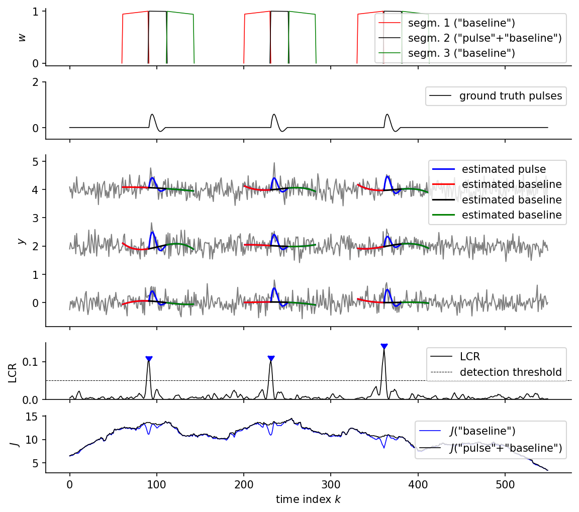
Demonstrates a spike detection algorithm that uses autonomous linear state space models together with exponentially decaying windows. The input is a multi-channel signal containing multiple spikes (sinusoidal cycles with decaying amplitude) with additive white Gaussian noise and a polynomial baseline.

The algorithm fits a spike model and a baseline model simultaneously using a CompositeCost, computes the Log-Cost Ratio (LCR) for each sample and channel, and identifies spike locations at LCR peaks.

Plot

Console Output

State-Space Matrix A is not upper triangular, cascade version can't be used. Defaulting to filter_form='parallel'.

Code

"""
Multi-Channel Spike Detection [ex112.0]
=======================================

Demonstrates a spike detection algorithm that uses autonomous linear state
space models together with exponentially decaying windows. The input is a
multi-channel signal containing multiple spikes (sinusoidal cycles with
decaying amplitude) with additive white Gaussian noise and a polynomial
baseline.

The algorithm fits a spike model and a baseline model simultaneously using
a [`CompositeCost`][lmlib.statespace.cost.CompositeCost], computes the Log-Cost Ratio (LCR) for each sample
and channel, and identifies spike locations at LCR peaks.

"""

import matplotlib.pyplot as plt
import numpy as np
import lmlib as lm
from scipy.linalg import block_diag
from scipy.signal import find_peaks

from lmlib.utils.generator import gen_conv, gen_sine, gen_exp, gen_pulse, gen_wgn, k_period_to_omega

# signal generation
K = 550
k = np.arange(K)
L = 3  # number of channels
spike_length = 20
spike_decay = 0.88
spike_locations = [100, 240, 370]
spike = gen_sine(spike_length, spike_length) * gen_exp(spike_length, spike_decay)
y_sp = gen_conv(gen_pulse(K, spike_locations), spike)
y = np.column_stack([0.8 * y_sp + gen_wgn(K, sigma=0.2, seed=10000 - l) for l in range(L)]).reshape(K, L)

# Segments
g_bl = 500
g_sp = 5000
len_sp = spike_length
len_bl = int(1.5 * spike_length)
segmentL = lm.Segment(a=-len_bl, b=-1, direction=lm.FORWARD, g=g_bl, delta=-1, label='left segment')
segmentC = lm.Segment(a=0, b=len_sp, direction=lm.BACKWARD, g=g_sp, label='center segment')
segmentR = lm.Segment(a=len_sp + 1, b=len_sp + 1 + len_bl, direction=lm.BACKWARD, g=g_bl, delta=len_sp, label='right segment')

# Model
alssm_sp = lm.AlssmSin(k_period_to_omega(spike_length), spike_decay)
alssm_bl = lm.AlssmPolyLegendre(poly_degree=3,a_seg=-len_bl,b_seg=len_sp+len_bl+1)

# Cost
F = [[0, 1, 0],
     [1, 1, 1]]
cost = lm.CompositeCost((alssm_sp, alssm_bl), (segmentL, segmentC, segmentR), F)

rls = lm.RLSAlssm(cost)
rls.filter(y)
H_sp = block_diag([[0], [1]], np.eye(alssm_bl.N))
xs_sp = rls.minimize_x(H_sp)
H_bl = np.vstack([np.zeros((alssm_sp.N, alssm_bl.N)), np.eye(alssm_bl.N)])
xs_bl = rls.minimize_x(H_bl)

# Error
J = rls.eval_errors(xs_sp)
J_bl = rls.eval_errors(xs_bl)
J_sum = np.sum(J, axis=-1) if J.ndim > 1 else J
J_bl_sum = np.sum(J_bl, axis=-1) if J.ndim > 1 else J_bl

lcr = -0.5 * np.log(J_sum / J_bl_sum)

LCR_THD = 0.05  # minimum log-cost ratio to detect a pulse in noise
peaks, _ = find_peaks(lcr, height=LCR_THD, distance=30)


# Window
wins = lm.Window.eval_y(cost, peaks, K, merged_seg=False, fill_value=np.nan)
for peak in peaks: #add a 0.0-value at the edge of the window for display purposes (np.nan is not plotted)
    wins[0,peak+segmentL.a-1] = 0.0
    wins[0,peak+segmentL.b+1] = 0.0
    wins[1,peak+segmentC.a-1] = 0.0
    wins[1,peak+segmentC.b+1] = 0.0
    wins[2,peak+segmentR.a-1] = 0.0
    wins[2,peak+segmentR.b+1] = 0.0

# Trajectories
trajs_baseline = lm.Trajectory.eval_y(cost, xs_sp, peaks, K, F=[[0, 0, 0], [1, 1, 1]], thd=0.01,merged_seg=False)
trajs_pulse = lm.Trajectory.eval_y(cost, xs_sp, peaks, K, F=[[0, 1, 0], [1, 1, 1]], thd=0.01)

# Plot
fig, axs = plt.subplots(5, 1, figsize=(9, 8), gridspec_kw={'height_ratios': [1, 1, 3, 1, 1]}, sharex='all')

axs[0].set(ylabel='$w$')
axs[0].plot(k, wins[0], color='r', lw=0.75, ls='-',  label=segmentL.label)
axs[0].plot(k, wins[1], color='k', lw=0.75, ls='-',  label=segmentC.label)
axs[0].plot(k, wins[2], color='g', lw=0.75, ls='-',  label=segmentR.label)
axs[0].legend(('segm. 1 ("baseline")', 'segm. 2 ("pulse"+"baseline")', 'segm. 3 ("baseline")'), loc=1)

# True Signals
axs[1].plot(range(K), y_sp, c='k', lw=0.8, label='ground truth pulses')
axs[1].set_ylim(-0.5, 2)
axs[1].legend(loc=1)

# Signals
OFFSETS = np.arange(L) * 2
axs[2].set(ylabel='$y$')
axs[2].plot(range(K), y + OFFSETS, c='tab:gray', lw=1)
axs[2].plot(range(K), trajs_pulse + OFFSETS, color='b', lw=1.5, linestyle="-", label=['estimated pulse'] + (L-1) * [''] )
for i, (traj_baseline,color) in enumerate(zip(trajs_baseline,['r','k','g'])):
    axs[2].plot(range(K), traj_baseline + OFFSETS, color=color, lw=1.5, linestyle="-", label=['estimated baseline'] + (L-1) * [''])
axs[2].legend(loc=1)

# LCR
axs[3].set(ylabel='LCR', ylim=[0, 0.15])
axs[3].plot(range(K), lcr, c='k', lw=0.8, label='LCR')
axs[3].scatter(peaks, lcr[peaks], marker=7, c='b')
axs[3].axhline(LCR_THD, color="black", linestyle="--", lw=0.5, label='detection threshold')
axs[3].legend(loc=1)

# Error
axs[4].plot(range(K), J_sum, c='b', lw=0.8, label='$J($' + '"baseline"' + '$)$')
axs[4].plot(range(K), J_bl_sum, c='k', lw=0.8, label='$J($' + '"pulse"+"baseline"' + '$)$')
axs[4].legend(loc=1)
axs[4].set(ylabel='$J$', xlabel='time index $k$')

for _ax in axs:
    _ax.spines['top'].set_visible(False)
    _ax.spines['right'].set_visible(False)

plt.show()