ECG Shape Detection [ex113.0]
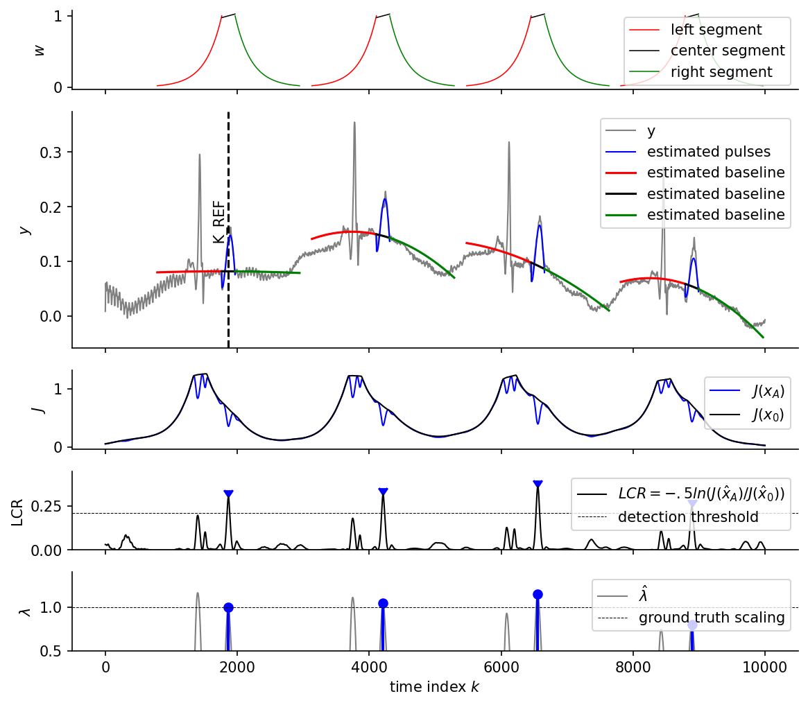
Detects a known reference shape in a single-channel electrocardiogram (ECG) signal using a template-matching approach based on ALSSMs.
A reference template is extracted from the signal at a known location
(K_REF). A polynomial ALSSM fits the template and every candidate
window in the signal; the Log-Cost Ratio (LCR) between a shape-model fit
and a flat-baseline fit is used to score each candidate. Peaks in the LCR
above LCR_THD are returned as detected beat locations.
Signal source: EECG_BASELINE_1CH_10S_FS2400HZ.csv (bundled library data).
Plot
Console Output
CompositeCost(label=n/a)
  └- ['AlssmPolyLegendre(A=[[1.0000000e+00 1.0000000e-02 1.5000000e-04 1.0002500e-02 5.0004375e-04] [0.0000000e+00 1.0000000e+00 3.0000000e-02 7.5000000e-04 3.0017500e-02] [0.0000000e+00 0.0000000e+00 1.0000000e+00 5.0000000e-02 1.7500000e-03] [0.0000000e+00 0.0000000e+00 0.0000000e+00 1.0000000e+00 7.0000000e-02] [0.0000000e+00 0.0000000e+00 0.0000000e+00 0.0000000e+00 1.0000000e+00]], C=[ 1.     0.    -0.5    0.     0.375], label=alssm-pulse)', 'AlssmPolyJordan(A=[[1. 1. 0.] [0. 1. 1.] [0. 0. 1.]], C=[1 0 0], label=alssm-baseline)'],
  └- ['Segment(a=-inf, b=-101, direction=fw, g=250, delta=-101, label=left segment)', 'Segment(a=-100, b=100, direction=fw, g=4000, delta=0, label=center segment)', 'Segment(a=101, b=inf, direction=bw, g=250, delta=101, label=right segment)']
H_A :  [[ 0.02660574  0.          0.          0.        ]
 [ 0.03474947  0.          0.          0.        ]
 [-0.05240043  0.          0.          0.        ]
 [-0.02329981  0.          0.          0.        ]
 [ 0.00817069  0.          0.          0.        ]
 [ 0.          1.          0.          0.        ]
 [ 0.          0.          1.          0.        ]
 [ 0.          0.          0.          1.        ]]
H_0 :  [[0. 0. 0.]
 [0. 0. 0.]
 [0. 0. 0.]
 [0. 0. 0.]
 [0. 0. 0.]
 [1. 0. 0.]
 [0. 1. 0.]
 [0. 0. 1.]]
Code
"""
ECG Shape Detection [ex113.0]
==============================

Detects a known reference shape in a single-channel electrocardiogram (ECG)
signal using a template-matching approach based on ALSSMs.

A reference template is extracted from the signal at a known location
(``K_REF``).  A polynomial ALSSM fits the template and every candidate
window in the signal; the Log-Cost Ratio (LCR) between a shape-model fit
and a flat-baseline fit is used to score each candidate.  Peaks in the LCR
above ``LCR_THD`` are returned as detected beat locations.

Signal source: ``EECG_BASELINE_1CH_10S_FS2400HZ.csv`` (bundled library data).
"""

import matplotlib.pyplot as plt
import numpy as np
from scipy.signal import find_peaks
from scipy.linalg import block_diag

import lmlib as lm
from lmlib.utils.generator import load_lib_csv

# --------------- loading test signal -----------------------
file_name = 'EECG_BASELINE_1CH_10S_FS2400HZ.csv'
K = 10000  # number of samples to process
y = load_lib_csv(file_name, K)

# --------------- parameters of example -----------------------
LCR_THD = 0.21  # minimum log-cost ratio to detect a pulse in noise

K_REF = 1865  # time index of reference shape

SHAPE_LEN_2 = 100  # 1/2 length of shape to be found
MIN_DIST = 1500  # minimal number of samples between two pulses

g_sp = 4000  # pulse window weight, effective sample number under the window # (larger value lead to a more rectangular-like windows while too large values might lead to nummerical instabilities in the recursive computations.)
g_bl = 250  # baseline window weight, effective sample number under the window (larger value leads to a wider window)

N1 = 3  # number of polynomial coefficient for baseline  Note: N>4 might leads to nummerical instabilities in the recursions
N2 = 5  # number of polynomial coefficient for spike. Note: N>4 might leads to  nummerical instabilities in the recursions.

# --------------- main -----------------------

# Defining segments with a left- resp. right-sided decaying window and a center segment with nearly rectangular window
segmentL = lm.Segment(a=-np.inf, b=-1 - SHAPE_LEN_2, direction=lm.FORWARD, g=g_bl, delta=-1 - SHAPE_LEN_2, label='left segment')
segmentC = lm.Segment(a=-SHAPE_LEN_2, b=SHAPE_LEN_2, direction=lm.FORWARD, g=g_sp, label='center segment')
segmentR = lm.Segment(a=SHAPE_LEN_2 + 1, b=np.inf, direction=lm.BACKWARD, g=g_bl, delta=SHAPE_LEN_2 + 1, label='right segment')

# Defining ALSSM models
alssm_baseline = lm.AlssmPolyJordan(poly_degree=N1 - 1, label="alssm-baseline")
#alssm_pulse = lm.AlssmPolyJordan(poly_degree=N2 - 1, label="alssm-pulse")
alssm_pulse = lm.AlssmPolyLegendre(poly_degree=N2 - 1, a_seg= segmentC.a, b_seg=segmentC.b, label="alssm-pulse")


# Defining the cost function (a so called composite cost = CCost)
# mapping matrix between models and segments (rows = models, columns = segments)
F = [[0, 1, 0],
     [1, 1, 1]]
cost = lm.CompositeCost((alssm_pulse, alssm_baseline), (segmentL, segmentC, segmentR), F)
print(cost)

# filter signal
rls = lm.RLSAlssm(cost, steady_state=False, backend='lfilter')
rls.filter(y)  # run recursions

xs = rls.minimize_x()  # unconstrained minimization
xs_ref = xs[K_REF]  # store state variables as reference pulse shape

H_A = np.transpose(block_diag([xs_ref[0:N2]], np.eye(N1)))  # constraints matrix to find pulses of same shape as the reference pulse
H_0 = np.transpose(np.hstack([np.zeros((N1, N2)), np.eye(N1)]))  # constraints matrix to test for no pulse (baseline only)

print("H_A : ", H_A)
print("H_0 : ", H_0)

xs_A = rls.minimize_x(H_A)
xs_0 = rls.minimize_x(H_0)

J_A = rls.eval_errors(xs_A)  # get SE (squared error) for hypothesis 1 (baseline + pulse)
J_0 = rls.eval_errors(xs_0)  # get SE (squared error)  for hypothesis 0 (baseline only) --> J0 should be a vector not a matrice

lcr = -0.5 * np.log(J_A / J_0)  # log-cost ratio computation

vs = rls.minimize_v(H_A)     # constrainted minimization (pulse scaling and baseline coefficients)
amp = vs[:, 0]               # optimal scaling of pulse over time

# find peaks
peaks, _ = find_peaks(lcr, height=LCR_THD, distance=MIN_DIST)

# --------------- plotting of results -----------------------
k = np.arange(K)

# Window
wins = lm.Window.eval_y(cost, peaks, K, merged_seg=False,thd=0.02,fill_value=np.nan)

# Trajectories
trajs_baseline = lm.Trajectory.eval_y(cost, xs_A, peaks, K, F=[[0, 0, 0], [1, 1, 1]], thd=0.02, merged_seg=False)
trajs_pulse    = lm.Trajectory.eval_y(cost, xs_A, peaks, K, F=[[0, 1, 0], [1, 1, 1]], thd=0.02)


fig, axs = plt.subplots(5, 1, figsize=(9, 8), gridspec_kw={'height_ratios': [1, 3, 1, 1, 1]}, sharex='all')

axs[0].plot(k, wins[0], color='r', lw=0.75, ls='-',  label=segmentL.label)
axs[0].plot(k, wins[1], color='k', lw=0.75, ls='-',  label=segmentC.label)
axs[0].plot(k, wins[2], color='g', lw=0.75, ls='-',  label=segmentR.label)
axs[0].set(ylabel='$w$')
axs[0].legend(loc='upper right')

axs[1].plot(k, y, color="gray", lw=1.0, label='y')
axs[1].axvline(x=K_REF, color='black', ls='--')
axs[1].text(K_REF, y[K_REF], ' K_REF', horizontalalignment='right', rotation=90)
axs[1].plot(range(K), trajs_pulse, color='b', lw=1.0, linestyle="-", label='estimated pulses')
for i, (traj_baseline,color) in enumerate(zip(trajs_baseline,['r','k','g'])):
    axs[1].plot(range(K), traj_baseline, color=color, lw=1.5, linestyle="-", label='estimated baseline')
axs[1].legend(loc='upper right')
axs[1].set(ylabel = '$y$')

axs[2].plot(k, J_A, lw=1.0, color='blue', label=r"$J(x_A)$")
axs[2].plot(k, J_0, lw=1.0, color='black', label=r"$J(x_0)$")
axs[2].legend(loc='upper right')
axs[2].set(ylabel = '$J$')

axs[3].plot(k, lcr, lw=1.0, color='black', label=r"$LCR = -.5 ln(J(\hat{x}_A) / J(\hat{x}_0))$")
axs[3].scatter(peaks, lcr[peaks], marker=7, c='b')
axs[3].axhline(LCR_THD, color="black", linestyle="--", lw=0.5, label='detection threshold')
axs[3].set_ylim(0.0, 0.45)
axs[3].set(ylabel = 'LCR')
axs[3].legend(loc='upper right')

axs[4].plot(k, amp, lw=1.0, color='gray', label=r'$\hat{\lambda}$')
_, stemlines, _ = axs[4].stem(peaks, amp[peaks], markerfmt="bo", basefmt=" ")
plt.setp(stemlines, 'linewidth', 2, 'color', 'blue')
axs[4].axhline(1.0, color="black", linestyle="--", lw=0.5, label='ground truth scaling')
axs[4].axhline(0, color="black", lw=0.5)
axs[4].legend(loc='upper right')
axs[4].set_ylim(0.5, 1.4)
axs[4].set(ylabel = r'$\lambda$', xlabel='time index $k$')

for _ax in axs:
    _ax.spines['top'].set_visible(False)
    _ax.spines['right'].set_visible(False)

plt.show()