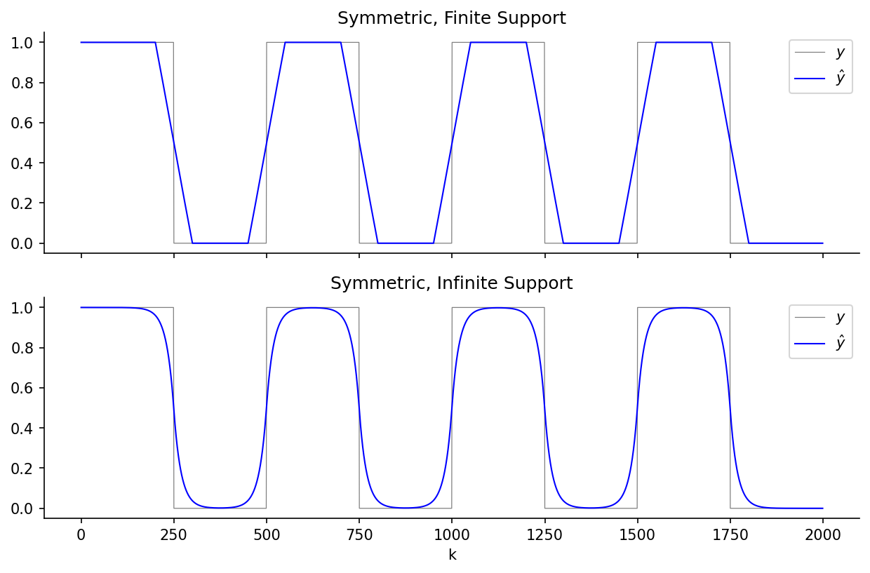
Symmetric Moving Average Filters with ALSSMs [ex121.0]

Applies a CompositeCost with a two-sided symmetric window as a symmetric moving average filter of length L=100.

A degree-0 polynomial ALSSM (i.e. a constant model) is combined with a forward left segment and a backward right segment of equal length. The resulting filter is equivalent to a finite-impulse-response (FIR) boxcar average, but is computed efficiently via the recursive ALSSM framework.

Plot

Code

"""
Symmetric Moving Average Filters with ALSSMs [ex121.0]
======================================================

Applies a [`CompositeCost`][lmlib.statespace.cost.CompositeCost] with a two-sided symmetric window as a
symmetric moving average filter of length L=100.

A degree-0 polynomial ALSSM (i.e. a constant model) is combined with a
forward left segment and a backward right segment of equal length.  The
resulting filter is equivalent to a finite-impulse-response (FIR) boxcar
average, but is computed efficiently via the recursive ALSSM framework.

"""

import matplotlib.pyplot as plt
import numpy as np
import lmlib as lm
from lmlib.utils.generator import gen_rect
import time

# --- Generating test signal ---
K = 2000
k = np.arange(K)
y = gen_rect(K, 500,250)

# Polynomial ALSSM
alssm_poly = lm.AlssmPoly(poly_degree=0, force_MC=False)

# --- Plot I: ALSSM Filtering - Finite Support Moving Average Filter ---
# Segments
segment_left = lm.Segment(a=-50, b=-1, direction=lm.FORWARD, g=1000)
segment_right = lm.Segment(a=0, b=49, direction=lm.BACKWARD, g=1000)

# Composite Cost
costs = lm.CompositeCost((alssm_poly,), (segment_left, segment_right), F=[[1, 1]])

# filter signal and take the approximation
rls = lm.RLSAlssm(costs, steady_state=False, calc_W=True)

# extracts filtered signal
y_hat_1 = rls.fit(y)

# --- Plot II: ALSSM Filtering - Symmetric Infinite Support Moving Average Filter ---
# Segments
segment_left = lm.Segment(a=-np.inf, b=-1, direction=lm.FORWARD, g=20)
segment_right = lm.Segment(a=0, b=np.inf, direction=lm.BACKWARD, g=20)

# Composite Cost
costs = lm.CompositeCost((alssm_poly,), (segment_left, segment_right), F=[[1, 1]])

# filter signal, take the approximation, and extracts filtered signal
rls = lm.RLSAlssm(costs, steady_state=False)
y_hat_2 = rls.fit(y)

# --- Plotting ----
fig, ax = plt.subplots(2, 1, sharex='all', figsize=(10,6))

ax[0].plot(k, y, lw=0.6, c='gray', label=rf'$y$')
ax[0].plot(k, y_hat_1, lw=1, c='b', label=r'$\hat{y}$')
ax[0].legend(loc='upper right')
ax[0].set_title('Symmetric, Finite Support')


ax[1].plot(k, y, lw=0.6, c='gray', label=rf'$y$')
ax[1].plot(k, y_hat_2, lw=1, c='b', label=r'$\hat{y}$')
ax[1].legend(loc='upper right')
ax[1].set_xlabel('k')
ax[1].set_title('Symmetric, Infinite Support')

for _ax in ax:
    _ax.spines['top'].set_visible(False)
    _ax.spines['right'].set_visible(False)

plt.show()