Symmetric and Non-Symmetric Polynomial Filters with Pascal Basis [ex122.0]

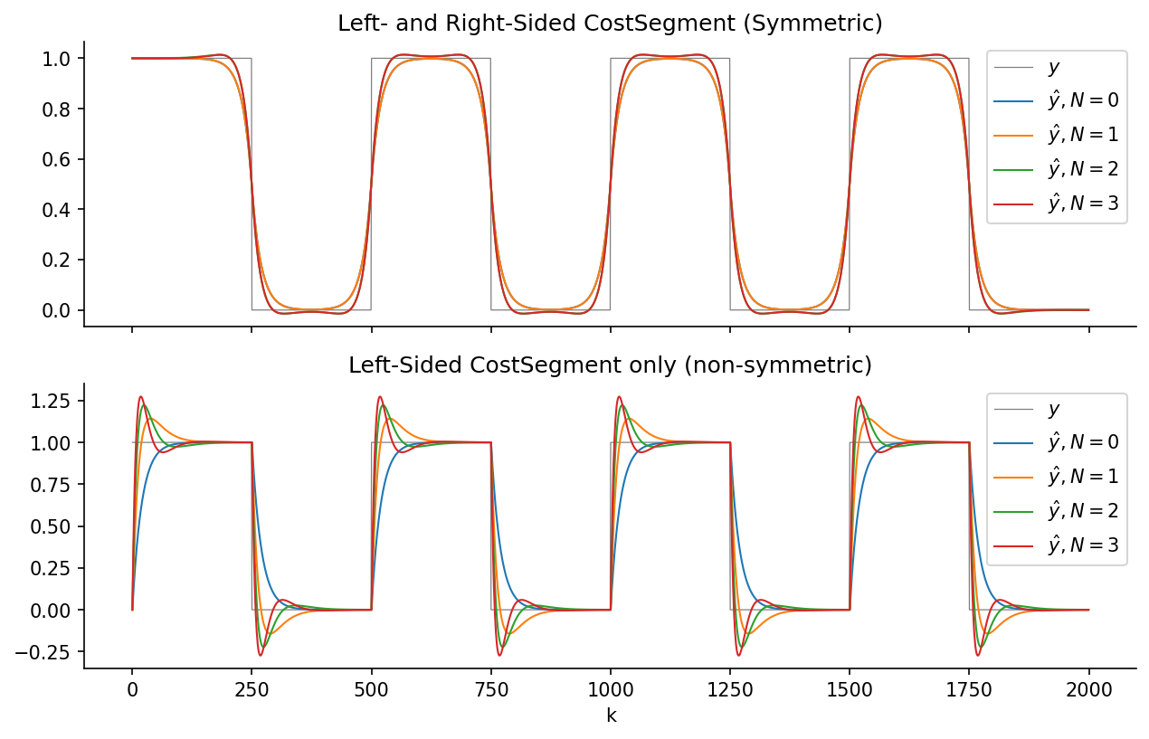
Applies CompositeCost instances with AlssmPoly of degrees 0 through 3 to a rectangular test signal.

Two filter configurations are shown for each polynomial degree:

• Symmetric filter — a forward left window and a backward right window of equal size, yielding a zero-phase (non-causal) smoother.
• Left (causal) filter — a single forward window on the left side only, yielding a causal, phase-delayed smoother.

Higher polynomial degrees follow the signal edges more closely but are more sensitive to noise away from transitions.

Plot

Code

"""
Symmetric and Non-Symmetric Polynomial Filters with Pascal Basis [ex122.0]
====================================================================

Applies [`CompositeCost`][lmlib.statespace.cost.CompositeCost] instances with [`AlssmPoly`][lmlib.statespace.model.AlssmPoly] of degrees
0 through 3 to a rectangular test signal.

Two filter configurations are shown for each polynomial degree:

* **Symmetric filter** — a forward left window and a backward right window
  of equal size, yielding a zero-phase (non-causal) smoother.
* **Left (causal) filter** — a single forward window on the left side only,
  yielding a causal, phase-delayed smoother.

Higher polynomial degrees follow the signal edges more closely but are more
sensitive to noise away from transitions.

"""

import matplotlib.pyplot as plt
import numpy as np
import lmlib as lm
from lmlib.utils.generator import gen_rect

# --- Generating test signal ---
K = 2000
k = np.arange(K)
y = gen_rect(K, 500, 250)

# --- ALSSM Filtering ---
y_hats_sym = []
y_hats_left = []

for i in range(0, 4):
    # Polynomial ALSSM
    alssm_poly = lm.AlssmPoly(poly_degree=i)

    # Segments
    segment_left = lm.Segment(a=-np.inf, b=-1, direction=lm.FORWARD, g=20)
    segment_right = lm.Segment(a=0, b=np.inf, direction=lm.BACKWARD, g=20)

    # -- Symmetric Filter --
    # Composite Cost
    costs = lm.CompositeCost((alssm_poly,), (segment_left, segment_right), F=[[1, 1]])

    # filter signal and take the approximation
    rls = lm.RLSAlssm(costs, steady_state=False)

    # extracts filtered signal
    y_hats_sym.append(rls.fit(y))

    # -- Left-Sided Filter --
    # CompositeCost
    costs = lm.CompositeCost((alssm_poly,), (segment_left, segment_right), F=[[1, 0]])

    # filter signal and take the approximation
    rls = lm.RLSAlssm(costs)

    # extracts filtered signal
    y_hats_left.append(rls.fit(y))

# --- Plotting ----
STYLES = ['tab:blue', 'tab:orange', 'tab:green', 'tab:red', 'tab:purple', 'tab:brown']
fig, ax = plt.subplots(2, sharex='all', figsize=(10, 6))
ax[0].plot(k, y, lw=0.6, c='gray', label=rf'$y$')
for (i, y_hat) in enumerate(y_hats_sym):
    ax[0].plot(k, y_hat, STYLES[i], lw=1, label=r'$\hat y, N=' + str(i) + '$')
ax[0].legend(loc='upper right')
ax[0].set_title('Left- and Right-Sided CostSegment (Symmetric)')

ax[1].plot(k, y, lw=0.6, c='gray', label=rf'$y$')
for (i, y_hat) in enumerate(y_hats_left):
    ax[1].plot(k, y_hat, STYLES[i], lw=1, label=r'$\hat y, N=' + str(i) + '$')
ax[1].legend(loc='upper right')
ax[1].set_title('Left-Sided CostSegment only (non-symmetric)')
ax[1].set_xlabel('k')

for _ax in ax:
    _ax.spines['top'].set_visible(False)
    _ax.spines['right'].set_visible(False)

plt.show()