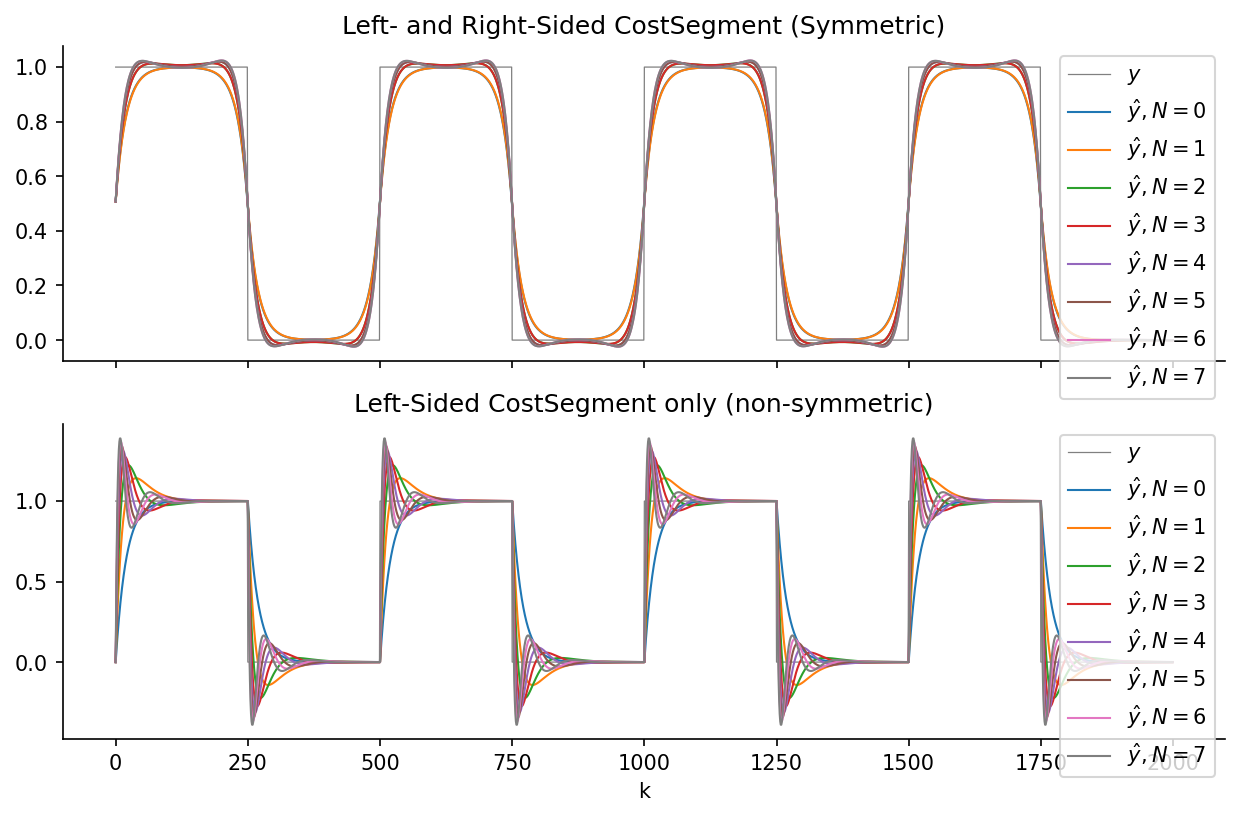
Symmetric and Non-Symmetric Polynomial Filters with Meixner Basis [ex122.1]

Applies CompositeCost instances with AlssmPolyMeixner of degrees 0 through 7 to a rectangular test signal.

The Meixner basis is orthogonal under the exponential (geometric) window weight, giving a well-conditioned Gram matrix for semi-infinite windows. This makes it the preferred polynomial basis for recursive least-squares filtering with exponential windows, especially at high polynomial degrees where the monomial (Pascal) basis of AlssmPoly becomes numerically ill-conditioned.

Two filter configurations are shown for each degree:

• Symmetric filter — forward left window and backward right window.
• Left (causal) filter — forward window on the left side only.

Plot

Code

"""
Symmetric and Non-Symmetric Polynomial Filters with Meixner Basis [ex122.1]
===========================================================================

Applies [`CompositeCost`][lmlib.statespace.cost.CompositeCost] instances with [`AlssmPolyMeixner`][lmlib.statespace.model.AlssmPolyMeixner] of
degrees 0 through 7 to a rectangular test signal.

The Meixner basis is orthogonal under the exponential (geometric) window
weight, giving a well-conditioned Gram matrix for semi-infinite windows.
This makes it the preferred polynomial basis for recursive least-squares
filtering with exponential windows, especially at high polynomial degrees
where the monomial (Pascal) basis of [`AlssmPoly`][lmlib.statespace.model.AlssmPoly] becomes numerically
ill-conditioned.

Two filter configurations are shown for each degree:

* **Symmetric filter** — forward left window and backward right window.
* **Left (causal) filter** — forward window on the left side only.

"""

import matplotlib.pyplot as plt
import numpy as np
import lmlib as lm
from lmlib.utils.generator import gen_rect

# --- Generating test signal ---
K = 2000
k = np.arange(K)
y = gen_rect(K, 500, 250)

# --- ALSSM Filtering ---
y_hats_sym = []
y_hats_left = []

for i in range(0, 8):

    # Segments
    segment_left = lm.Segment(a=-np.inf, b=-1, direction=lm.FORWARD, g=20)
    segment_right = lm.Segment(a=0, b=np.inf, direction=lm.BACKWARD, g=20)

    # Polynomial ALSSM
    alssm_L = lm.AlssmPolyMeixner(i, segment=segment_left)
    alssm_R = lm.AlssmPolyMeixner(i, segment=segment_right)

    # -- Symmetric Filter --
    # Composite Cost
    F =  [[1,0],[0,1]]
    cost    = lm.CompositeCost((alssm_L, alssm_R), (segment_left, segment_right), F=F)

    # filter signal and take the approximation
    rls = lm.RLSAlssm(cost)

    # extracts filtered signal
    y_hats_sym.append(rls.fit(y,H=cost.spline_H(max_continuity=i),eval_alssm_weights=[0,1]))   

    # -- Left-Sided Filter --
    # CompositeCost
    costs = lm.CompositeCost((alssm_L,), (segment_left, ), F=[[1]])

    # filter signal and take the approximation
    rls = lm.RLSAlssm(costs)

    # extracts filtered signal
    y_hats_left.append(rls.fit(y))

# --- Plotting ----
fig, ax = plt.subplots(2, sharex='all', figsize=(10, 6))
ax[0].plot(k, y, lw=0.6, c='gray', label=r'$y$')
for (i, y_hat) in enumerate(y_hats_sym):
    ax[0].plot(k, y_hat, lw=1, label=r'$\hat y, N=' + str(i) + '$')
ax[0].legend(loc='upper right')
ax[0].set_title('Left- and Right-Sided CostSegment (Symmetric)')

ax[1].plot(k, y, lw=0.6, c='gray', label=r'$y$')
for (i, y_hat) in enumerate(y_hats_left):
    ax[1].plot(k, y_hat,  lw=1, label=r'$\hat y, N=' + str(i) + '$')
ax[1].legend(loc='upper right')
ax[1].set_title('Left-Sided CostSegment only (non-symmetric)')
ax[1].set_xlabel('k')

for _ax in ax:
    _ax.spines['top'].set_visible(False)
    _ax.spines['right'].set_visible(False)


plt.show()