Multi-Channel Symmetric Signal Filter [ex123.0]

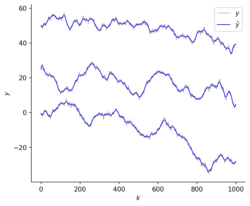
Applies a CompositeCost with a symmetric two-sided window as a symmetric linear filter to a multi-channel signal.

A degree-5 polynomial ALSSM is fitted over equal-length left and right windows. The same model is applied in parallel to all channels using the multi-channel (MC) output form of the ALSSM. Each channel is minimized individually.

Plot

Code

"""
Multi-Channel Symmetric Signal Filter [ex123.0]
===============================================

Applies a [`CompositeCost`][lmlib.statespace.cost.CompositeCost] with a symmetric two-sided window as a
symmetric linear filter to a multi-channel signal.

A degree-5 polynomial ALSSM is fitted over equal-length left and right
windows.  The same model is applied in parallel to all channels using the
multi-channel (MC) output form of the ALSSM. Each channel is minimized individually.

"""

import matplotlib.pyplot as plt
import numpy as np
import lmlib as lm
from lmlib.utils.generator import gen_rand_walk

# --- Generating test signal ---
K = 1000
seeds = [130, 150, 200]
NCH = len(seeds)
y = np.column_stack([gen_rand_walk(K, seed=s) for s in seeds])


# --- ALSSM Filtering ---
# Polynomial ALSSM
alssm_poly = lm.AlssmPoly(poly_degree=5)

# Segments
segment_left = lm.Segment(a=-50, b=-1, direction=lm.FW, g=10)
segment_right = lm.Segment(a=0, b=50, direction=lm.BW, g=10)

# Composite Cost
costs = lm.CompositeCost((alssm_poly,), (segment_left, segment_right), F=[[1, 1]])

# filter signal and take the approximation
rls = lm.RLSAlssm(costs, steady_state=False)

# extracts filtered signals
y_hat = rls.fit(y)

# --- Plotting ----
fig, ax = plt.subplots(1, 1, sharex='all', figsize=(6, 5), )
OFFSETS = np.arange(NCH ) * 25

ax.plot(y + OFFSETS,     lw=0.6, c='gray', label=[r'$y$'] + ['_nolegend_'] * (NCH - 1) )
ax.plot(y_hat + OFFSETS, lw=1,   c='b',    label=[r'$\hat{{y}}$'] + ['_nolegend_'] * (NCH - 1))
ax.legend(loc='upper right')

ax.set(xlabel='$k$',ylabel='$y$')

ax.spines['top'].set_visible(False)
ax.spines['right'].set_visible(False)


plt.show()