Multi-Scale Polynomial (Savitzky-Golay) Smoothing: Causal vs Centered [ex125.0]
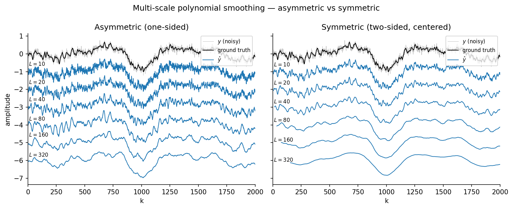
Smooths a noisy single-channel EEG signal at a dyadic family of window lengths \(L \in \{10, 20, 40, 80, 160, 320\}\) with polynomial ALSSMs, and shows the two standard windowing choices side by side:
- Causal (left) — a one-sided (left-sided) BACKWARD window (\(a = 0\), \(b = L-1\), total length \(L\)). It uses only current and past samples, so it can run online, but it introduces a scale-dependent lag (visible as the smoothed trace shifting to the right at large \(L\)).
- Centered (right) — a symmetric, zero-lag window (\(a = -L/2\), \(b = L/2-1\), total length \(L\), i.e. \(L/2\) samples on each side), the choice Savitzky-Golay smoothing normally uses. It is non-causal (needs future samples) but introduces no lag.
For each mode the example contrasts two mathematically equivalent ways of obtaining the multi-scale result:
- Per-scale RLS — a fresh
RLSAlssmover aCompositeCostis run for every scale, so the \(O(K)\) recursion is evaluated once per scale. - State reuse — the recursion is run only once at the base scale and each larger scale is built by dyadic composition of the filter state \((\xi, W)\).
For the causal window a length-\(2L\) window is two stacked length-\(L\) windows; the trailing one is propagated to the common reference by \(A^{L}\) and re-weighted by the segment decay \(\gamma^{L}\):
For the centered window, with the half-shift \(h = L/2\), a length-\(2L\) centered window is two length-\(L\) windows centered at \(k-h\) and \(k+h\); each is propagated to the common reference \(k\) by \(A^{\pm h}\) and re-weighted:
(The scalar weights are \(\gamma_\mathrm{fwd}^{\pm h}\); for a FORWARD segment lmlib uses \(\gamma_\mathrm{fwd} = 1/(1 - 1/g)\), so \(\gamma_\mathrm{fwd}^{\pm h} = \gamma^{\mp h}\) with \(\gamma = 1 - 1/g\).) For each mode the script checks that both methods agree numerically and reports the speed-up of state reuse.
Plot
Data
This example uses the following data file(s):
Console Output
=== CAUSAL: numerical equivalence (interior k in [300, 1700)) ===
   L=  10   max|per-scale - reuse| = 6.883e-14
   L=  20   max|per-scale - reuse| = 8.356e-09
   L=  40   max|per-scale - reuse| = 7.878e-11
   L=  80   max|per-scale - reuse| = 8.544e-11
   L= 160   max|per-scale - reuse| = 1.399e-09
   L= 320   max|per-scale - reuse| = 1.603e-08
   worst over all scales = 1.603e-08
   timing over 30 runs (M=6 scales, K+overlap=2800):
     Method 1 per-scale RLS : mean   18.83 ms  best   18.70 ms
     Method 2 xi reuse      : mean    2.58 ms  best    2.54 ms
     mean speed-up          :  7.30x

=== CENTERED: numerical equivalence (interior k in [300, 1700)) ===
   L=  10   max|per-scale - reuse| = 7.105e-15
   L=  20   max|per-scale - reuse| = 1.504e-10
   L=  40   max|per-scale - reuse| = 7.242e-12
   L=  80   max|per-scale - reuse| = 7.095e-12
   L= 160   max|per-scale - reuse| = 5.052e-11
   L= 320   max|per-scale - reuse| = 1.526e-09
   worst over all scales = 1.526e-09
   timing over 30 runs (M=6 scales, K+overlap=2800):
     Method 1 per-scale RLS : mean   18.99 ms  best   18.79 ms
     Method 2 xi reuse      : mean    2.72 ms  best    2.67 ms
     mean speed-up          :  6.99x
Code
r"""
Multi-Scale Polynomial (Savitzky-Golay) Smoothing: Causal vs Centered [ex125.0]
===============================================================================

Smooths a noisy single-channel EEG signal at a dyadic family of window lengths
$L \in \{10, 20, 40, 80, 160, 320\}$ with polynomial ALSSMs, and shows the two
standard windowing choices side by side:

* **Causal (left)** — a **one-sided (left-sided) BACKWARD window** ($a = 0$,
  $b = L-1$, total length $L$). It uses only current and past samples, so it can
  run online, but it introduces a scale-dependent lag (visible as the smoothed
  trace shifting to the right at large $L$).
* **Centered (right)** — a **symmetric, zero-lag window** ($a = -L/2$,
  $b = L/2-1$, total length $L$, i.e. $L/2$ samples on each side), the choice
  Savitzky-Golay smoothing normally uses. It is non-causal (needs future
  samples) but introduces no lag.

For each mode the example contrasts two mathematically equivalent ways of
obtaining the multi-scale result:

* **Per-scale RLS** — a fresh [`RLSAlssm`][lmlib.statespace.rls.RLSAlssm] over a
  [`CompositeCost`][lmlib.statespace.cost.CompositeCost] is run for every scale,
  so the $O(K)$ recursion is evaluated once per scale.
* **State reuse** — the recursion is run only once at the base scale and each
  larger scale is built by dyadic composition of the filter state $(\xi, W)$.

For the **causal** window a length-$2L$ window is two stacked length-$L$ windows;
the trailing one is propagated to the common reference by $A^{L}$ and re-weighted
by the segment decay $\gamma^{L}$:

$$
\xi_{2L}[k] = \xi_L[k] + \gamma^{L}\, \xi_L[k+L]\, A^{L}, \qquad
W_{2L} = W_L + \gamma^{L}\, A^{L\mathsf{T}} W_L\, A^{L}.
$$

For the **centered** window, with the half-shift $h = L/2$, a length-$2L$
centered window is two length-$L$ windows centered at $k-h$ and $k+h$; each is
propagated to the common reference $k$ by $A^{\pm h}$ and re-weighted:

$$
\xi_{2L}[k] = \gamma^{-h}\, \xi_L[k+h]\, A^{h} + \gamma^{+h}\, \xi_L[k-h]\, A^{-h}, \qquad
W_{2L} = \gamma^{-h}\, A^{h\mathsf{T}} W_L\, A^{h} + \gamma^{+h}\, A^{-h\mathsf{T}} W_L\, A^{-h}.
$$

(The scalar weights are $\gamma_\mathrm{fwd}^{\pm h}$; for a FORWARD segment lmlib
uses $\gamma_\mathrm{fwd} = 1/(1 - 1/g)$, so $\gamma_\mathrm{fwd}^{\pm h} =
\gamma^{\mp h}$ with $\gamma = 1 - 1/g$.) For each mode the script checks that
both methods agree numerically and reports the speed-up of state reuse.
"""
import time
import numpy as np
import matplotlib.pyplot as plt
import lmlib as lm
from lmlib.utils.generator import gen_wgn, load_csv_mc

# ----------------------------------------------------------------------
# Load Data
# ----------------------------------------------------------------------
data = load_csv_mc("amananandrai_eeg_s00.csv")  # EEG, fs=500Hz
# channels: Fp1, Fp2, F3, F4, F7, F8, T3, T4, C3, C4, T5, T6, P3, P4, O1, O2, Fz, Cz, Pz.
CH       = 0
K        = 2000
k        = np.arange(K)
OVERLAP  = 800                       # headroom for the widest window
data = data[:, CH]
data = data / np.nanmax(np.abs(data))
kstart = 24500
y_true = data[kstart:kstart + K + OVERLAP]                    # ground truth (noise-free)
y      = y_true + gen_wgn(K + OVERLAP, sigma=0.1, seed=3142)   # noisy observation

# ----------------------------------------------------------------------
# Model and scales
# ----------------------------------------------------------------------
N      = 4                                   # poly_degree = 3
G      = 800
GAMMA  = 1.0 - 1.0 / G
BASE   = 10
SCALES = [BASE * 2 ** j for j in range(6)]   # 10, 20, 40, 80, 160, 320


def build_rls(L, mode):
    """One-segment RLSAlssm for scale L, causal (one-sided) or centered."""
    if mode == 'causal':
        seg = lm.Segment(a=0, b=L - 1, direction=lm.BACKWARD, g=G)
    else:  # 'centered'
        seg = lm.Segment(a=-L // 2, b=L // 2 - 1, direction=lm.FORWARD, g=G)
    cost = lm.CompositeCost((lm.AlssmPolyJordan(poly_degree=N - 1),), (seg,), F=[[1]])
    return lm.RLSAlssm(cost, steady_state=True, backend='lfilter')


# ----------------------------------------------------------------------
# METHOD 1 -- per-scale RLS (the usual concept, no reuse of intermediate results)
# ----------------------------------------------------------------------
def method_per_scale(y, mode):
    out = {}
    for L in SCALES:
        out[L] = build_rls(L, mode).fit(y, output='y_hat')
    return out


# ----------------------------------------------------------------------
# METHOD 2 -- single recursion + dyadic xi/W reuse
# ----------------------------------------------------------------------
def method_reuse(y, mode):
    rls0 = build_rls(BASE, mode)
    A    = np.asarray(rls0._cost_terms.alssms[0].A, dtype=float)
    C    = np.asarray(rls0._cost_terms.alssms[0].C, dtype=float)
    rls0.filter(y)
    xi   = np.asarray(rls0.xi).copy()
    W    = np.asarray(rls0.W).copy()
    out  = {BASE: xi @ np.linalg.inv(W) @ C}
    L = BASE
    while L * 2 <= SCALES[-1]:
        if mode == 'causal':
            AL = np.linalg.matrix_power(A, L)          # A^{L}
            gL = GAMMA ** L
            v  = K + OVERLAP - L
            xitilde = np.full_like(xi, np.nan)
            xitilde[:v] = xi[:v] + gL * (xi[L:L + v] @ AL)
            Wtilde      = W + gL * (AL.T @ W @ AL)
        else:  # 'centered'
            h  = L // 2
            Ah = np.linalg.matrix_power(A, h)          # A^{+h}
            Ai = np.linalg.inv(Ah)                     # A^{-h}
            gp = GAMMA ** (-h)                          # weight for the k+h half
            gm = GAMMA ** (h)                           # weight for the k-h half
            v  = K + OVERLAP - h
            xitilde = np.full_like(xi, np.nan)
            xitilde[h:v] = gp * (xi[2 * h:v + h] @ Ah) + gm * (xi[0:v - h] @ Ai)
            Wtilde       = gp * (Ah.T @ W @ Ah) + gm * (Ai.T @ W @ Ai)

        out[L * 2] = xitilde @ np.linalg.inv(Wtilde) @ C
        xi, W, L = xitilde, Wtilde, L * 2
    return out


# ----------------------------------------------------------------------
# Equivalence + timing, per mode
# ----------------------------------------------------------------------
def benchmark(fn, mode, reps):
    fn(y, mode)                                   # warm-up
    t = np.array([(lambda t0: (fn(y, mode), time.perf_counter() - t0)[1])(time.perf_counter())
                  for _ in range(reps)]) * 1e3
    return t.mean(), t.std(), t.min()


REPS = 30
results = {}
for mode in ('causal', 'centered'):
    A_out, B_out = method_per_scale(y, mode), method_reuse(y, mode)
    results[mode] = B_out
    sl = slice(300, K - 300)
    print(f"=== {mode.upper()}: numerical equivalence (interior k in [{sl.start}, {sl.stop})) ===")
    for L in SCALES:
        print(f"   L={L:4d}   max|per-scale - reuse| = "
              f"{np.nanmax(np.abs(A_out[L][sl] - B_out[L][sl])):.3e}")
    worst = max(np.nanmax(np.abs(A_out[L][sl] - B_out[L][sl])) for L in SCALES)
    print(f"   worst over all scales = {worst:.3e}")
    t1 = benchmark(method_per_scale, mode, REPS)
    t2 = benchmark(method_reuse, mode, REPS)
    print(f"   timing over {REPS} runs (M={len(SCALES)} scales, K+overlap={K + OVERLAP}):")
    print(f"     Method 1 per-scale RLS : mean {t1[0]:7.2f} ms  best {t1[2]:7.2f} ms")
    print(f"     Method 2 xi reuse      : mean {t2[0]:7.2f} ms  best {t2[2]:7.2f} ms")
    print(f"     mean speed-up          : {t1[0] / t2[0]:5.2f}x\n")

# ----------------------------------------------------------------------
# Verification plot: causal (left) vs centered (right), shared axes
# ----------------------------------------------------------------------
offset = 1
fig, axs = plt.subplots(1, 2, figsize=(11, 4.5), sharex='all', sharey='all')
titles = {'causal': 'Asymmetric (one-sided)',
          'centered': 'Symmetric (two-sided, centered)'}

for ax, mode in zip(axs, ('causal', 'centered')):
    B_out = results[mode]
    ax.plot(k, y[k], lw=0.5, alpha=0.5, c='gray', label='$y$ (noisy)')
    ax.plot(k, y_true[k], lw=1.0, c='black', label='ground truth')
    for i, L in enumerate(SCALES):
        ax.plot(k, B_out[L][k] - (i + 1) * offset, lw=1.0, c='tab:blue',
                label=r'$\hat y$' if i == 0 else None)
        ax.text(8, np.nanmax(B_out[L][0:200]) - (i + 1) * offset + 0.05, f"$L={L}$", size=8)
    ax.set_xlim([0, K])
    ax.set_title(titles[mode])
    ax.set_xlabel('k')
    ax.legend(loc='upper right', fontsize=8)
    for s in ('top', 'right'):
        ax.spines[s].set_visible(False)

axs[0].set_ylabel('amplitude')

fig.suptitle('Multi-scale polynomial smoothing — asymmetric vs symmetric')
fig.tight_layout()
plt.show()