Edge Detection [ex401.1]

Example published in [Waldmann2022] as Example 1.

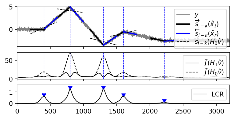
Illustrates edge detection using a Two-Sided Line Model (TSLM) that scores each sample by the Log-Cost Ratio (LCR) between a Continuous constraint (shared offset and matching slopes on both sides) and a Straight constraint (single global line). Peaks in the LCR above a threshold indicate slope discontinuities (edges).

This application-level example uses the TSLM creator class for conciseness. For the equivalent educational step-by-step construction see example ex401.0.

Plot

Code

r"""
Edge Detection [ex401.1]
====================================================
Example published in [\[Waldmann2022\]](../../../bibliography.md#waldmann2022) as Example 1.

Illustrates edge detection using a Two-Sided Line Model (TSLM) that scores
each sample by the Log-Cost Ratio (LCR) between a ``Continuous`` constraint
(shared offset and matching slopes on both sides) and a ``Straight`` constraint
(single global line).  Peaks in the LCR above a threshold indicate slope
discontinuities (edges).

This application-level example uses the [`TSLM`][lmlib.statespace.applications.TSLM]
creator class for conciseness.  For the equivalent educational step-by-step
construction see example ``ex401.0``.

"""

import numpy as np
import matplotlib.pyplot as plt
from scipy.signal import find_peaks

import lmlib as lm
from lmlib.utils.generator import gen_slopes, gen_wgn

# --- Generate Test Signal ---
fs = 1  # (Relative) Sampling rate
K = 3200 * fs  # Length of Test signal
k = range(K)
ks = np.multiply([400, 800, 1300, 1600, 2200], fs)
deltas = [0, 5, -8.5, 3, -2]
y = gen_slopes(K, ks, deltas) + 1.0 * gen_wgn(K, sigma=0.2, seed=3141)

# 0 -- Parameters -----
a = (-200 * fs)  # Left segment length
b = (200 * fs) - 1  # Right segment length
gl = 70.0 * fs  # Left segment window decay
gr = 70.0 * fs  # Right segment window decay

# 1 -- Two-Sided Line Model (TSLM)-----

# cost model to detect events
ccost = lm.TSLM.create_cost(ab=(a, b), gs=(gl, gr))

# the following two costs are for visulatization purpose only - and not needed to solve the problem
cost_l = lm.TSLM.create_cost(ab=(a, 1), gs=(gl, gr))
cost_r = lm.TSLM.create_cost(ab=(-2, b), gs=(gl, gr))

# Applying Filters
rls = lm.RLSAlssm(ccost, steady_state=False)
rls.filter(y)

rls_l = lm.RLSAlssm(cost_l, steady_state=False)
rls_l.filter(y)
rls_r = lm.RLSAlssm(cost_r, steady_state=False)
rls_r.filter(y)

# Filter
x_hat_line = rls.minimize_x(lm.TSLM.H_Straight)
x_hat_edge_l = rls_l.minimize_x()
x_hat_edge_r = rls_r.minimize_x()
x_hat_edge = rls.minimize_x(lm.TSLM.H_Continuous)

# Square Error and LCR
error_edge_l = rls_l.eval_errors(x_hat_edge_l)
error_edge_r = rls_r.eval_errors(x_hat_edge_r)
error_edge = rls.eval_errors(x_hat_edge)
error_line = rls.eval_errors(x_hat_line)
lcr = -1 / 2 * np.log(np.divide(error_edge, error_line))

# Find LCR peaks with minimal distance and height
peaks, _ = find_peaks(lcr, height=.1, distance=200 * fs)

# Evaluate trajectories (for plotting only)
trajs_edge = lm.Trajectory.eval_y(ccost, x_hat_edge, peaks, K, merged_seg=False)
trajs_line = lm.Trajectory.eval_y(ccost, x_hat_line, peaks, K, merged_seg=False)

wins = lm.Window.eval_y(ccost, peaks, K, merged_seg=False)
# -- PLOTTING --
_, axs = plt.subplots(3, 1, figsize=(6, 3.2), gridspec_kw={'height_ratios': [1.5, 1.0, 0.7]}, sharex='all')
nax = 0  # current subplot index

t = np.array(list(k))
axs[nax].plot(t, y, lw=1, c='gray', label='$y$', zorder=0)
axs[nax].plot(t, trajs_edge[0, :], c='k', lw=2, ls='-', zorder=1, label=r'$\overrightarrow{s}_{i-k}(\hat x_\ell)$')
axs[nax].plot(t, trajs_edge[1, :], c='b', lw=2, ls='-', zorder=1, label=r'$\overleftarrow{s}_{i-k}(\hat x_r)$')
axs[nax].plot(t, trajs_line[0, :], c='k', lw=1, ls='--', zorder=1, label=r'${s}_{i-k}(H_0 \hat v)$')
axs[nax].plot(t, trajs_line[1, :], c='k', lw=1, ls='--', zorder=1)
axs[nax].scatter(peaks[0], x_hat_edge[peaks[0], 0], marker='.', c='k', s=20.0)

for xp in peaks:
    axs[nax].axvline(x=xp, ls='--', c='b', lw=0.5)

axs[nax].legend(loc='upper right', labelspacing=-0.0)
axs[nax].set_ylim(bottom=min(y), top=max(y))
nax += 1

# Cost plot
kswitch = ks[1]
kdif = ks[1] - kswitch
axs[nax].plot(k, error_edge, c='xkcd:black', label=r'$\tilde J(H_1 \hat v)$', lw=1.0)
axs[nax].plot(k, error_line, c='xkcd:black', ls='--', label=r'$\tilde J(H_0 \hat v)$', lw=1.0)

axs[nax].legend(loc='upper right', labelspacing=-0.0)
for xp in peaks:
    axs[nax].axvline(x=xp, ls='--', c='b', lw=0.5)

nax += 1
# LCR plot
axs[nax].plot(k, np.concatenate((lcr[kdif:], lcr[0:kdif],)), c='xkcd:black', label='LCR', lw=1.0)
axs[nax].legend(loc='center right')
axs[nax].scatter(peaks, lcr[peaks], marker=7, c='b')
axs[nax].set_ylim(-0.05, 1.6)
axs[nax].set_xlim(left=0.0, right=3200.0)

plt.subplots_adjust(bottom=0.21)

plt.show()