Notch Detection in ABP Signal [ex402.0]
Example published in [Waldmann2022] as Example 2.
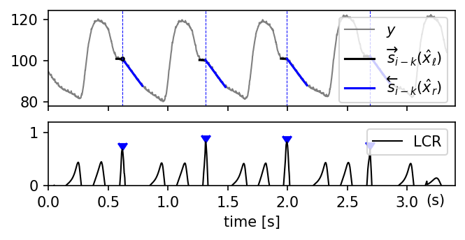
Arterial blood pressure (ABP) signals typically show a dicrotic notch in
the descending slope, marking the end of the systolic cycle. This example
detects these notches using a Two-Sided Line Model (TSLM) that compares
a Continuous line fit (no slope change) against a Free fit (independent
slopes on each side) via the Log-Cost Ratio (LCR). A peak in the LCR signals
the presence of a notch.
Plot
Data
This example uses the following data file(s):
Code
r"""
Notch Detection in ABP Signal [ex402.0]
====================================================
Example published in [\[Waldmann2022\]](../../../bibliography.md#waldmann2022) as Example 2.

Arterial blood pressure (ABP) signals typically show a dicrotic notch in
the descending slope, marking the end of the systolic cycle.  This example
detects these notches using a Two-Sided Line Model (TSLM) that compares
a ``Continuous`` line fit (no slope change) against a ``Free`` fit (independent
slopes on each side) via the Log-Cost Ratio (LCR).  A peak in the LCR signals
the presence of a notch.

"""

import numpy as np
import matplotlib.pyplot as plt
from scipy.signal import find_peaks

import lmlib as lm
from lmlib.utils.generator import gen_wgn, load_csv

# Linear Constraints
H_Free = np.array(
    [[1, 0, 0, 0],  # x_A,left : offset of left line
     [0, 1, 0, 0],  # x_B,left : slope of left line
     [0, 0, 1, 0],  # x_A,right : offset of right line
     [0, 0, 0, 1]])  # x_B,right : slope of right line

H_Continuous = np.array(
    [[1, 0, 0],  # x_A,left : offset of left line
     [0, 1, 0],  # x_B,left : slope of left line
     [1, 0, 0],  # x_A,right : offset of right line
     [0, 0, 1]])  # x_B,right : slope of right line

H_Straight = np.array(
    [[1, 0],  # x_A,left : offset of left line
     [0, 1],  # x_B,left : slope of left line
     [1, 0],  # x_A,right : offset of right line
     [0, 1]])  # x_B,right : slope of right line

H_Horizontal = np.array(
    [[1],  # x_A,left : offset of left line
     [0],  # x_B,left : slope of left line
     [1],  # x_A,right : offset of right line
     [0]])  # x_B,right : slope of right line

H_Left_Horizontal = np.array(
    [[1, 0],  # x_A,left : offset of left line
     [0, 0],  # x_B,left : slope of left line
     [1, 0],  # x_A,right : offset of right line
     [0, 1]])  # x_B,right : slope of right line

H_Right_Horizontal = np.array(
    [[1, 0],  # x_A,left : offset of left line
     [0, 1],  # x_B,left : slope of left line
     [1, 0],  # x_A,right : offset of right line
     [0, 0]])  # x_B,right : slope of right line

H_Peak = np.array(
    [[1, 0],  # x_A,left : offset of left line
     [0, 1],  # x_B,left : slope of left line
     [1, 0],  # x_A,right : offset of right line
     [0, -1]])  # x_B,right : slope of right line

H_Step = np.array(
    [[1, 0],  # x_A,left : offset of left line
     [0, 0],  # x_B,left : slope of left line
     [0, 1],  # x_A,right : offset of right line
     [0, 0]])  # x_B,right : slope of right line


# Implementation of Two-Sided Line Model (TSLM)
# y: input signal vector
# a,b: left and right sided interval border (in number of samples)
# gl, gr: left and right sided exponential window weight (defines exponential decay factor gamma)

def J_TSLM(y, a, b, gl, gr):
    # Set up Composite Cost Model using two ALSSMs and exponentially decaying windows
    #
    #         ---->     <----
    #      --------------------
    #  A_L |   c_L  |    0    |
    #      --------------------
    #  A_R |   0    |    c_R  |
    #      --------------------
    #      :        :         :
    #     a=-80     0        b=20

    alssm_left = lm.AlssmPoly(poly_degree=1)  # A_L, c_L
    alssm_right = lm.AlssmPoly(poly_degree=1)  # A_R, c_R
    segment_left = lm.Segment(a=a, b=-1, direction=lm.FORWARD, g=gl)
    segment_right = lm.Segment(a=0, b=b, direction=lm.BACKWARD, g=gr)
    F = [[1, 0], [0, 1]]  # mixing matrix, turning on and off models per segment (1=on, 0=off)
    costs = lm.CompositeCost((alssm_left, alssm_right), (segment_left, segment_right), F)

    return costs


# Constants
K = 2000  # number of samples
sigma = 0.015  # Adding Gaussian Noise
fs = 600  # Sampling Frequency [Hz]
k = range(K)

# -- TEST SIGNAL --
y = load_csv('cerebral-vasoreg-diabetes-heaad-up-tilt_day1-s0030DA-noheader.csv', K,
             channel=3)  # probably sampled at 600Hz
y = y + gen_wgn(K, sigma, seed=233453)  # Add Gaussian Noise

# 1 -- Onset Detection with Two-Sided Line Model (TSLM) -----
costs = J_TSLM(y, -30, 100, gl=180, gr=180)

# Filter
rls = lm.RLSAlssm(costs)
rls.filter(y)

# constraint minimization
x_hat_H1 = rls.minimize_x(H_Left_Horizontal)
x_hat_H0 = rls.minimize_x(H_Straight)

y = y[k]
x_hat_H1 = x_hat_H1[k]
x_hat_H0 = x_hat_H0[k]

# Square Error and LCR
error_H1 = rls.eval_errors(x_hat_H1)
error_H0 = rls.eval_errors(x_hat_H0)
lcr = -1 / 2 * np.log(np.divide(error_H1, error_H0))

# Find LCR peaks with minimal distance and height
peaks, _ = find_peaks(lcr, height=0.5, distance=300)

# Evaluate trajectories (for plotting only)

trajs_edge = lm.Trajectory.eval_y(costs, x_hat_H1, peaks, K, merged_seg=False)
trajs_line = lm.Trajectory.eval_y(costs, x_hat_H0, peaks, K, merged_seg=False)

wins = lm.Window.eval_y(costs, peaks, K, merged_seg=False)

# -- PLOTTING --
_, axs = plt.subplots(2, 1, figsize=(5, 2.5), gridspec_kw={'height_ratios': [1.5, 1]}, sharex='all')

nax = 0
t = np.array(list(k)) / fs
axs[nax].plot(t, y, lw=1.0, c='gray', label='$y$', zorder=0)
axs[nax].plot(t, trajs_edge[0, :], c='k', lw=1.5, ls='-', zorder=1, label=r'$\overrightarrow{s}_{i-k}(\hat x_\ell)$')
axs[nax].plot(t, trajs_edge[1, :], c='b', lw=1.5, ls='-', zorder=1, label=r'$\overleftarrow{s}_{i-k}(\hat x_r)$')
axs[nax].scatter(peaks[0] / fs, x_hat_H1[peaks[0], 0], marker='.', c='k', s=20.0)

# axs[nax].axhline(x=peaks, ymin=plt.ylim()[0], ymax=plt.ylim()[1])
for peak in peaks / fs:
    axs[nax].axvline(x=peak, ls='--', c='b', lw=0.5)

# axs[nax].scatter(peaks, y[peaks], marker=7, c='b')
axs[nax].legend(loc=1)
nax += 1

axs[nax].plot(t, lcr, lw=1.0, c='k', label='LCR')
axs[nax].scatter(peaks / fs, lcr[peaks], marker=7, c='b')
axs[nax].legend(loc='upper right', labelspacing=-0.0)
axs[nax].set_ylim(-0.0, 1.2)
axs[nax].set(xlabel='time [s]')
plt.gcf().text(0.845, 0.135, '(s)')

axs[nax].set_xlim(left=0.0, right=3.4)
plt.subplots_adjust(bottom=0.21)

plt.show()