ECG P, T Wave Onset and Peak Detection [ex403.0]¶

Example published in [Waldmann2022] as Example 3.

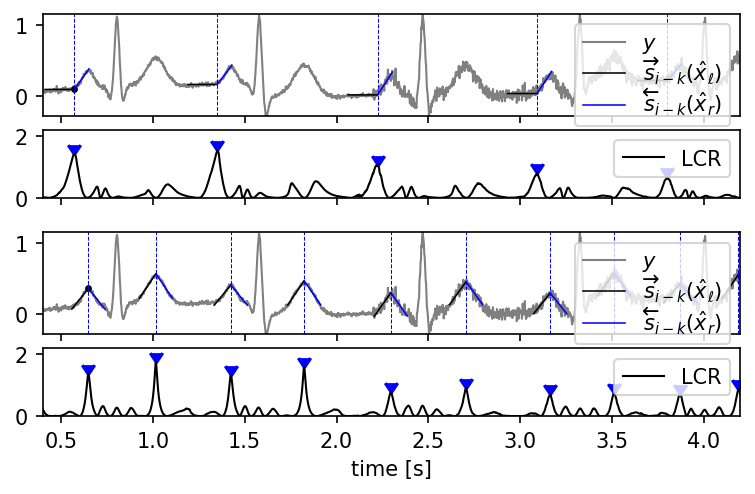
A common task in cardiology is to accurately measure the onsets and peaks of P and T waves in electrocardiography (ECG) signals. This example demonstrates a Two-Sided Line Model (TSLM) approach for extracting these fiducial points.

Two separate TSLM cost functions (costs_A for onsets, costs_B for peaks) are applied to a noisy ECG signal. Candidate locations are identified by LCR peaks, and onset / peak positions are refined by selecting the extremum within a neighbourhood of each peak.

Plot¶

Plot

Data¶

This example uses the following data file(s):

ECG_001-nohead.csv

Code¶

r"""
ECG P, T Wave Onset and Peak Detection [ex403.0]
================================================
Example published in [\[Waldmann2022\]](../../../bibliography.md#waldmann2022) as Example 3.

A common task in cardiology is to accurately measure the onsets and peaks
of P and T waves in electrocardiography (ECG) signals.  This example
demonstrates a Two-Sided Line Model (TSLM) approach for extracting these
fiducial points.

Two separate TSLM cost functions (``costs_A`` for onsets, ``costs_B`` for
peaks) are applied to a noisy ECG signal.  Candidate locations are identified
by LCR peaks, and onset / peak positions are refined by selecting the extremum
within a neighbourhood of each peak.

"""

import numpy as np
import matplotlib.pyplot as plt
from scipy.signal import find_peaks

import lmlib as lm
from lmlib.utils.generator import gen_wgn, load_csv

# Constants
K = 2200  # number of samples
sigma = 0.015  # Adding Gaussian Noise
fs = 500  # Sampling Frequency [Hz]
k = range(K)

# load alternative ECG signal
y = load_csv('ECG_001-nohead.csv', K, channel=1)

y = y + gen_wgn(K, sigma, seed=233453) * np.concatenate((np.ones(K // 2), 3 * np.ones(K - K // 2)))

# cost model to detect events
costs_A = lm.TSLM.create_cost(ab=(-80, 40), gs=(80, 80))

# Filter
rls_A = lm.RLSAlssm(costs_A)
rls_A.filter(y)

# constraint minimization
x_hat_H1_A = rls_A.minimize_x(lm.TSLM.H_Left_Horizontal)
x_hat_H0_A = rls_A.minimize_x(lm.TSLM.H_Horizontal)

# Square Error and LCR
error_edge_A = rls_A.eval_errors(x_hat_H1_A)
error_line_A = rls_A.eval_errors(x_hat_H0_A)
lcr_A = -1 / 2 * np.log(np.divide(error_edge_A, error_line_A))

# Find LCR peaks with minimal distance and height
peaks_A, _ = find_peaks(lcr_A, height=.25, distance=300)

# Evaluate trajectories (for plotting only)
trajs_edge_A = lm.Trajectory.eval_y(costs_A, x_hat_H1_A, peaks_A, K, merged_seg=False)
trajs_line_A = lm.Trajectory.eval_y(costs_A, x_hat_H0_A, peaks_A, K, merged_seg=False)

# (B) -- T wave peak Detection -----
costs_B = lm.TSLM.create_cost(ab=(-45, 45), gs=(80, 80))

# Filter
rls_B = lm.RLSAlssm(costs_B)
rls_B.filter(y)

# constraint minimization
x_hat_H1_B = rls_B.minimize_x(lm.TSLM.H_Peak)
x_hat_H0_B = rls_B.minimize_x(lm.TSLM.H_Horizontal)

# Square Error and LCR
error_edge_B = rls_B.eval_errors(x_hat_H1_B)
error_line_B = rls_B.eval_errors(x_hat_H0_B)
lcr = -1 / 2 * np.log(np.divide(error_edge_B, error_line_B))

# Find LCR peaks with minimal distance and height
peaks_B, _ = find_peaks(lcr, height=.25, distance=150)

# Evaluate trajectories (for plotting only)
trajs_edge_B = lm.Trajectory.eval_y(costs_B, x_hat_H1_B, peaks_B, K, merged_seg=False)
trajs_line_B = lm.Trajectory.eval_y(costs_B, x_hat_H0_B, peaks_B, K, merged_seg=False)

wins = lm.Window.eval_y(costs_B, peaks_B, K, merged_seg=False)
# -- PLOTTING --
_, axs = plt.subplots(5, 1, figsize=(6, 4), gridspec_kw={'height_ratios': [1.5, 1, 0.1, 1.5, 1]}, sharex='all')
nax = 0

# ----- p onset -----
t = np.array(list(k)) / fs

axs[nax].plot(t, y, lw=1.0, c='gray', label='$y$', zorder=0)
if True:
    axs[nax].plot(t, trajs_edge_A[0, :], c='k', lw=.75, ls='-', zorder=1, label=r'$\overrightarrow{s}_{i-k}(\hat x_\ell)$')
    axs[nax].plot(t, trajs_edge_A[1, :], c='b', lw=.75, ls='-', zorder=1, label=r'$\overleftarrow{s}_{i-k}(\hat x_r)$')
    axs[nax].scatter(peaks_A[0] / fs, x_hat_H1_A[peaks_A[0], 0], marker='.', c='k', s=20.0)

for xp in peaks_A / fs:
    axs[nax].axvline(x=xp, ls='--', c='b', lw=0.5)

# axs[nax].scatter(peaks_A, y[peaks_A], marker=7, c='b')
axs[nax].legend(loc='upper right', labelspacing=-0.0)
axs[nax].set_ylim(bottom=min(y), top=max(y))
nax += 1

axs[nax].plot(t, lcr_A, lw=1.0, c='k', label='LCR')
axs[nax].scatter(peaks_A / fs, lcr_A[peaks_A], marker=7, c='b')
axs[nax].legend(loc=1)
axs[nax].set_ylim(bottom=-0, top=2.2)

nax += 1
axs[nax].set_visible(False)
nax += 1

t = np.array(list(k)) / fs

axs[nax].plot(t, y, lw=1.0, c='gray', label='$y$', zorder=0)
if True:
    axs[nax].plot(t, trajs_edge_B[0, :], c='k', lw=.75, ls='-', zorder=1, label=r'$\overrightarrow{s}_{i-k}(\hat x_\ell)$')
    axs[nax].plot(t, trajs_edge_B[1, :], c='b', lw=.75, ls='-', zorder=1, label=r'$\overleftarrow{s}_{i-k}(\hat x_r)$')
    axs[nax].scatter(peaks_B[1] / fs, x_hat_H1_B[peaks_B[1], 0], marker='.', c='k', s=20.0)

for xp in peaks_B / fs:
    axs[nax].axvline(x=xp, ls='--', c='b', lw=0.5)

axs[nax].legend(loc='upper right', labelspacing=-0.0)
axs[nax].set_ylim(bottom=min(y), top=max(y))
nax += 1

axs[nax].plot(t, lcr, lw=1.0, c='k', label='LCR')
axs[nax].scatter(peaks_B / fs, lcr[peaks_B], marker=7, c='b')
axs[nax].legend(loc=1)
axs[nax].set_ylim(bottom=0, top=2.2)
axs[nax].set_xlim(left=.4, right=4.2)
axs[nax].set(xlabel='time [s]')

nax += 1
plt.subplots_adjust(bottom=0.21)

plt.show()