Overview of Two-Sided Line Model (TSLM) Applications [ex404.0]

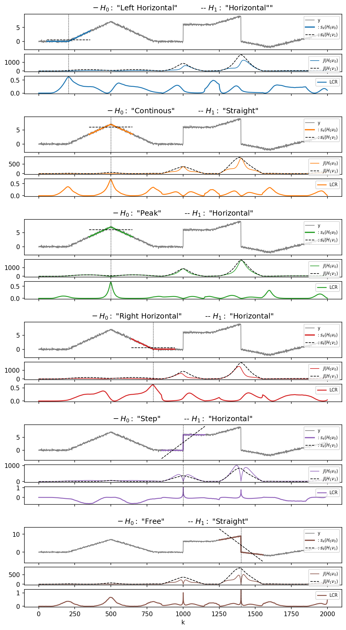
Compares multiple Two-Sided Line Model (TSLM) constraint types on a piecewise-linear test signal; cf. [Waldmann2022].

For each pair of hypothesis constraints (H0, H1), the Log-Cost Ratio (LCR) is computed and plotted. The constraint pairs tested are:

• Left Horizontal vs. Horizontal
• Continuous vs. Straight
• Peak vs. Horizontal
• Right Horizontal vs. Horizontal
• Step vs. Straight
• Free vs. Straight

Each LCR highlights a different class of changepoints (edges, peaks, steps, etc.) in the signal.

Plot

Console Output

CompositeCost(label=TSLM) 
  └- ['AlssmPoly(A=[[1 1] [0 1]], C=[1 0], label=left line model)', 'AlssmPoly(A=[[1 1] [0 1]], C=[1 0], label=right line model)'], 
  └- ['Segment(a=-150, b=-1, direction=fw, g=50, delta=0, label=left segment)', 'Segment(a=0, b=150, direction=bw, g=50, delta=0, label=right segment)']

Code

r"""
Overview of Two-Sided Line Model (TSLM) Applications [ex404.0]
===============================================================

Compares multiple Two-Sided Line Model (TSLM) constraint types on a
piecewise-linear test signal; cf. [\[Waldmann2022\]](../../../bibliography.md#waldmann2022).

For each pair of hypothesis constraints (H0, H1), the Log-Cost Ratio
(LCR) is computed and plotted.  The constraint pairs tested are:

* Left Horizontal vs. Horizontal
* Continuous vs. Straight
* Peak vs. Horizontal
* Right Horizontal vs. Horizontal
* Step vs. Straight
* Free vs. Straight

Each LCR highlights a different class of changepoints (edges, peaks, steps,
etc.) in the signal.

"""

import lmlib as lm
import numpy as np
import matplotlib.pyplot as plt
from lmlib.utils import gen_slopes, gen_wgn

K = 2000
ks = [200, 500, 800, 1000, 1001, 1200, 1400, 1401, 1600, 2000]
deltas = [0, 7, -7, 0, 6, 0, 3, -9, -2, 5]
y = gen_slopes(K, ks, deltas) + gen_wgn(K, 2e-1, seed=31415921)

H0s_Labels = ['"Left Horizontal"',       '"Continous"',        '"Peak"',             '"Right Horizontal"',       '"Step"',          '"Free"']
H0s        = [lm.TSLM.H_Left_Horizontal, lm.TSLM.H_Continuous, lm.TSLM.H_Peak,       lm.TSLM.H_Right_Horizontal, lm.TSLM.H_Step,    lm.TSLM.H_Free]

H1s_Labels = ['"Horizontal""',           '"Straight"',         '"Horizontal"',       '"Horizontal"',            '"Horizontal"',      '"Straight"']
H1s        = [lm.TSLM.H_Horizontal,      lm.TSLM.H_Straight,   lm.TSLM.H_Horizontal, lm.TSLM.H_Horizontal,      lm.TSLM.H_Straight,  lm.TSLM.H_Straight]

M = len(H0s_Labels)
colors0 = plt.colormaps['tab20'].colors[::2]

a = -150
b = 150
cost = lm.TSLM.create_cost(ab=(a, b), gs=(50, 50))
rls = lm.RLSAlssm(cost)
print(cost)

fig, axs = plt.subplots(4*M-1, sharex='all', figsize=(8, 14), gridspec_kw={'height_ratios': [2.0, 1, 1]+[0.8, 2.0, 1, 1]*(M-1)})
fig.subplots_adjust(left=0.08, right=.98, top=.98, bottom=0.02)

i = 0 # iteration counter
iaxs = 0 # axis counter
for H0, H1, c0, name0, name1 in zip(H0s, H1s, colors0,  H0s_Labels, H1s_Labels):
    rls.filter(y)
    xs_0 = rls.minimize_x(H=H0)
    xs_1 = rls.minimize_x(H=H1)

    J_0 = rls.eval_errors(xs_0)
    J_1 = rls.eval_errors(xs_1)

    LCR = -0.5 * np.log10(J_0 / J_1)

    ks_range = np.arange(K)
    ks_max = ks_range[[np.nanargmax(LCR)]]

    trajs_0 = lm.Trajectory.eval_y(cost, xs_0, ks_max, K, merged_ks=True, merged_seg=True)
    trajs_1 = lm.Trajectory.eval_y(cost, xs_1[ks_max], ks_max, K)

    # add spacer between subplots   
    if i>0:
        axs[iaxs].set_visible(False)
        iaxs += 1

    axs[iaxs].set_title("─ $H_0:$ "+name0 + '          ' + "-- $H_1:$ "+name1)
    axs[iaxs].plot(y, c=(0.5,)*3, lw=1.0, label='y')
    axs[iaxs].plot(trajs_0, c=c0,  lw=2.0, label=r': $s_k(H_0 v_0)$')
    axs[iaxs].plot(trajs_1, c='k', ls='--', lw=1.00, label=r': $s_k(H_1 v_1)$')
    axs[iaxs].legend(loc=1, fontsize=7)
    axs[iaxs].axvline(x=ks_max, ls='--', c='k', lw=0.5)
    iaxs += 1

    axs[iaxs].plot(ks_range, J_0[ks_range], c=c0, ls='-', lw=1, label='$J(H_0 v_0)$')
    axs[iaxs].plot(ks_range, J_1[ks_range], c='k', ls='--', lw=1, label='$J(H_1 v_1)$')
    axs[iaxs].axvline(x=ks_max, ls='--', c='k', lw=0.5)
    axs[iaxs].legend(loc=1, fontsize=7)
    iaxs += 1

    axs[iaxs].plot(ks_range, LCR[ks_range], c=c0, ls='-', lw=1.5, label= 'LCR')
    axs[iaxs].legend(loc=1, fontsize=7)
    axs[iaxs].axvline(x=ks_max, ls='--', c='k', lw=0.5)
    iaxs += 1
    i+=1

axs[-1].set_xlabel('k')

plt.show()