Matched Filter in Low-Dimensional ALSSM Feature Space [ex502.0]

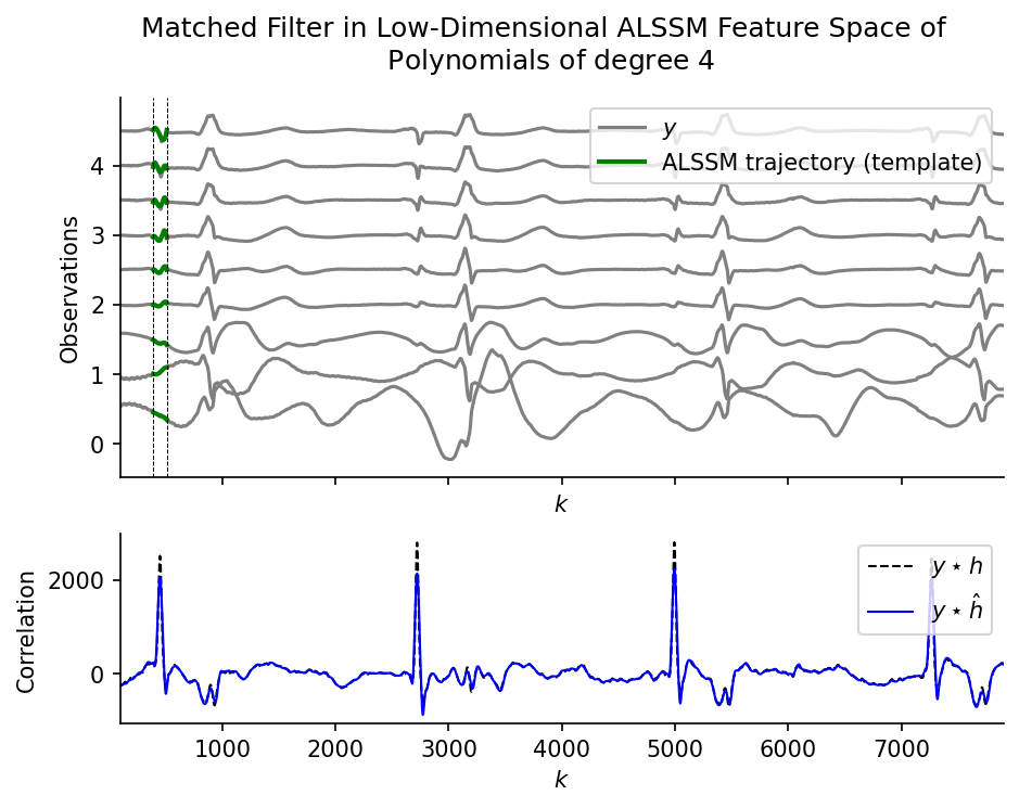
Implements a matched filter using ALSSM signal approximations (polynomial basis) to significantly increase processing speed compared to a direct sample-domain matched filter.

A reference template is extracted from a 9-channel ECG signal and projected onto the Legendre polynomial basis via AlssmPolyLegendre. The matched filter response is computed as an inner product of the template state vector with each signal window's state vector, which runs in \(O(N_\text{states})\) per sample instead of \(O(N_\text{template})\).

Author(s): Christof Baeriswyl

Plot

Code

r"""
Matched Filter in Low-Dimensional ALSSM Feature Space [ex502.0]
===============================================================

Implements a matched filter using ALSSM signal approximations (polynomial
basis) to significantly increase processing speed compared to a direct
sample-domain matched filter.

A reference template is extracted from a 9-channel ECG signal and projected
onto the Legendre polynomial basis via [`AlssmPolyLegendre`][lmlib.statespace.model.AlssmPolyLegendre].  The
matched filter response is computed as an inner product of the template
state vector with each signal window's state vector, which runs in
$O(N_\text{states})$ per sample instead of $O(N_\text{template})$.

Author(s): Christof Baeriswyl
"""
import numpy as np
import matplotlib.pyplot as plt
from matplotlib import gridspec
import time
import lmlib as lm
from lmlib.utils import load_lib_csv_mc

# -- 0. Loading Test signal ---
K = 8000  # number of samples to process
file_name = 'EECG_FILT_9CH_10S_FS2400HZ.csv'
K_REF = 450  # Location of reference template (Index of shape to correlate with)
y_mc = load_lib_csv_mc(file_name, K, channels=[0, 1, 2, 3, 4, 5, 6, 7, 8])
NOFCH = y_mc.shape[1]

k = range(K)

# -- 1. Polynomial ALSSM model for later signal approximation --
a = -60  # length of shape to correlate with, i.e., uses samples {K_REF+a, ..., K_REF+b} as the correlation template
b = 60
pd = 4  # polynomial order (number of coefficients) 
alssm = lm.AlssmPolyLegendre(poly_degree=pd, a_seg=a,b_seg=b) #can also be lm.AlssmPolyJordan(poly_degree=pd, label='Alssm')
segment = lm.Segment(a=a, b=b, direction=lm.BACKWARD, g=400)
cost = lm.CostSegment(alssm, segment)

# -- 2. Project observations (and the template) to ALSSM feature space --
rls_y = lm.RLSAlssm(cost, backend='lfilter')
rls_y.filter(y_mc)  # Transform observations

xs_hat = rls_y.minimize_x()  # get transformed observations
xs_h = xs_hat[K_REF]  # get correlation tempalte

# -- 3a. Get ALSSM Template of Matched filter
Ryy = np.cov(y_mc.T)
xs_h_matched = np.linalg.inv(Ryy) @ xs_h
# additionally, we may scale (normalize) the filter, such that E(noise) = 1. 
# alpha = 1/np.sqrt(np.sum(np.matmul(xs_h, np.matmul(np.linalg.inv(Ryy), xs_h_matched.T)), axis=(0,1)))
# xs_h_matched = alpha * xs_h_matched 


# -- 3b. Get Template of Matched filter in Sample Space (for comparison only)
h_mc = y_mc[K_REF + a:K_REF + b + 1, :]
Ryy = np.cov(y_mc.T)
h_mc_matched = (np.linalg.inv(Ryy) @ h_mc.T).T
# additionally, we may scale (normalize) the filter, such that E(noise) = 1. 
# alpha = 1/np.sqrt(np.sum(np.matmul(h_mc,np.matmul(np.linalg.inv(Ryy),h_mc_matched.T)),axis=(0,1)))
# h_mc_matched =  alpha * h_mc_matched 


# -- 4. Fast convolution in ALSSM feature space (channel-wise) --
# xi-only filter for the convolution: no W / kappa and no steady state needed.
rls = lm.RLSAlssm(cost, steady_state=False, calc_W=False, calc_kappa=False, backend='lfilter')

# Matched filtering in ALSSM feature space: filter y and contract the
# per-sample state with the matched template. The multichannel template
# (NOFCH, N) is summed over channels automatically.
corr_alssm = rls.convolve(y_mc, xs_h_matched)

# -- 5. Standard convolution in sample space (channel-wise) (for comparison) --
corr_native = np.zeros(y_mc.shape[0])
for j in range(NOFCH):
    corr_native[-a:-a + K - (b - a)] += np.correlate(y_mc[:, j], h_mc_matched[:, j], 'valid')

# -- 6.  Plotting --
template_trajectory = lm.Trajectory.eval_y(cost, xs_h, K_REF, K)

_, axs = plt.subplots(2, 1, figsize=(7, 5), gridspec_kw={'height_ratios': [2, 1]}, sharex='all')
nax = 0
offsets = (np.arange(NOFCH, 0, -1) * .5)

# Observation 
axs[nax].set(xlabel='$k$', ylabel=r'$y$')
axs[nax].plot(k, y_mc + offsets, c='gray',  label=['$y$'] + [''] * (NOFCH - 1))
axs[nax].plot(k, template_trajectory + offsets, '-', c='g', lw=2.0, label=['ALSSM trajectory (template)'] + [''] * (NOFCH - 1))
axs[nax].axvline(K_REF + a, color="black", linestyle="--", lw=0.5)
axs[nax].axvline(K_REF + b, color="black", linestyle="--", lw=0.5)
#axs[nax].axvline(K_REF, color="tab:red", linestyle=":", lw=1.0)
axs[nax].legend(loc='upper right')
axs[nax].set(ylabel='Observations')
ch_labels = ['Obs. CH {}'.format(i) for i in range(NOFCH, 0, -1)]
# axs[nax].legend(ch_labels)

# Convolution
nax += 1
axs[nax].set(xlabel='$k$')
axs[nax].plot(k, corr_native, ls='--', c='k', lw=1, label=r'$y \star  h$')
axs[nax].plot(k, corr_alssm,  ls='-',  c='b', lw=1, label=r'$y \star \hat h$')
axs[nax].legend(loc='upper right')
axs[nax].set(ylabel='Correlation')

axs[nax].set_xlim(100, K - 100)

for _ax in axs:
    _ax.spines['top'].set_visible(False)
    _ax.spines['right'].set_visible(False)

plt.suptitle('Matched Filter in Low-Dimensional ALSSM Feature Space of \n Polynomials of degree $' + str(pd) + '$')
plt.show()