Convolution and Correlation in Low-Dimensional ALSSM Feature Space [ex503.0]

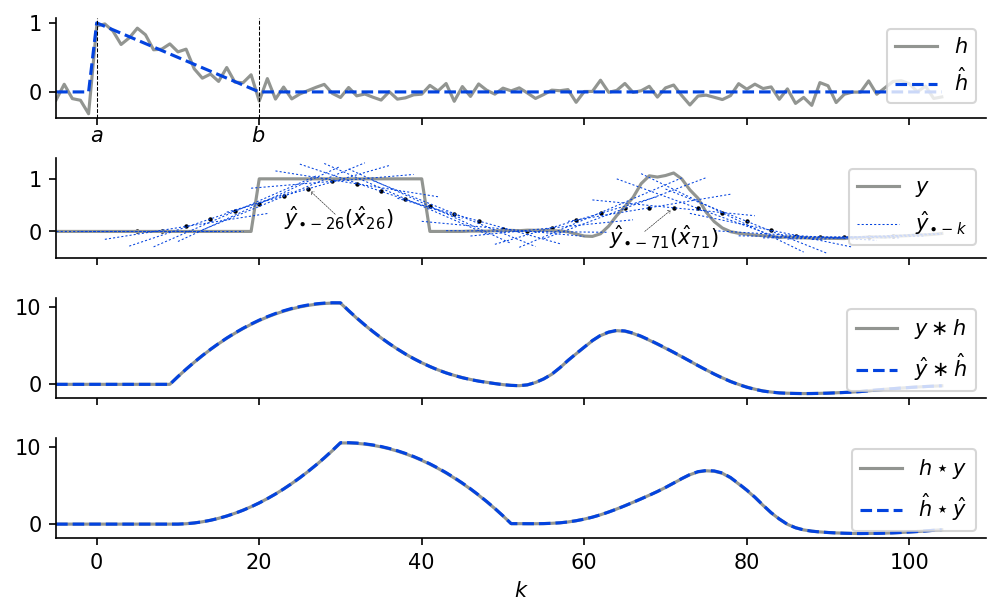
Computes the convolution, cross-correlation, and auto-correlation of a signal \(y\) with a reference filter \(h\) directly in a low-dimensional ALSSM feature space instead of in the original sample space.

Both the signal and the filter are projected onto a polynomial basis through an AlssmPolyJordan model that is fitted recursively with RLSAlssm. Each operation then reduces to an inner product of the compact state vectors (via a precomputed cross-window matrix \(W\)), which is faster than the corresponding direct sample-domain computation. The native numpy convolution and correlation are plotted alongside the ALSSM results for comparison.

Plot

Code

r"""
Convolution and Correlation in Low-Dimensional ALSSM Feature Space [ex503.0]
============================================================================

Computes the convolution, cross-correlation, and auto-correlation of a signal
$y$ with a reference filter $h$ directly in a low-dimensional ALSSM feature
space instead of in the original sample space.

Both the signal and the filter are projected onto a polynomial basis through an
[`AlssmPolyJordan`][lmlib.statespace.model.AlssmPolyJordan] model that is fitted
recursively with [`RLSAlssm`][lmlib.statespace.rls.RLSAlssm]. Each operation
then reduces to an inner product of the compact state vectors (via a precomputed
cross-window matrix $W$), which is faster than the corresponding direct
sample-domain computation. The native ``numpy`` convolution and correlation are
plotted alongside the ALSSM results for comparison.
"""
import numpy as np
import matplotlib.pyplot as plt
import lmlib as lm
from numpy.linalg import matrix_power as mpow
from scipy.signal import resample_poly

def calc_W12_1d_1segment(segment,alssm1,alssm2):
    A1 = alssm1.A
    C1 = alssm1.C.reshape(1,alssm1.C.shape[0])
    A2 = alssm2.A
    C2 = alssm2.C.reshape(1,alssm2.C.shape[0])
    W = np.zeros((A1.shape[0],A2.shape[1]),dtype=float)
    k0=0
    for i in range(segment.a+k0,segment.b+k0+1):
        W += segment.gamma**(i-k0) * mpow(A1,i-k0).T @ C1.T @ C2 @ mpow(A2,i-k0)
    return W


K = 110  # number of samples to process
koffset = -5
k = range(+koffset,K+koffset)
y_sc = np.zeros(K)
y_sc[20-koffset:41-koffset] = 1

file_name = 'EECG_FILT_9CH_10S_FS2400HZ.csv'
y_secg = lm.utils.load_lib_csv_mc(file_name, 3000+100, channels=[0])

# resample ECG
fs_original = 2400  # Original sampling frequency
fs_new = 200  # New sampling frequency
gcd = np.gcd(fs_original, fs_new)
up = fs_new // gcd
down = fs_original // gcd
y_secg_resampled = resample_poly(y_secg, up, down)
y_secg_resampled = y_secg_resampled/np.max(y_secg_resampled)

y_sc[50:] = y_secg_resampled[50:110] - y_secg_resampled[50]
y_noise = np.random.normal(0.0, 0.01, y_sc.shape[0])


# -- 1. Polynomial ALSSM model for later signal approximation --
a = -10  # length of shape to correlate with, i.e., uses samples {K_REF+a, ..., K_REF+b} as the correlation template
b = 10
polydegree = 1  # polynomial order (number of coefficients)
alssm = lm.AlssmPolyJordan(poly_degree=polydegree, label='Alssm')
segment = lm.Segment(a=a, b=b, direction=lm.BACKWARD, g=1000)
segmentinv = lm.Segment(a=a, b=b, direction=lm.FORWARD, g=1000)
cost = lm.CostSegment(alssm, segment)
alssminv = lm.Alssm(np.linalg.inv(alssm.A), alssm.C)
costinv = lm.CostSegment(alssminv, segmentinv)

# -- 2. Project observations to ALSSM feature space --
# rls objects used only for convolve() need xi only (no W / kappa, no steady
# state); convolve() filters the signal internally.
rls_yreversed = lm.RLSAlssm(cost, steady_state=False, calc_W=False, calc_kappa=False)

rls_y = lm.RLSAlssm(cost, steady_state=True)
rls_y.filter(y_sc)  # Transform observations
x_hat_y = rls_y.minimize_x()  # get transformed observations
y_hat = cost.eval_alssm_output(x_hat_y)  # signal reconstruction using ALSSM approximation (for illustration only)
# dedicated xi-only filter for the convolution/correlation of y_sc
rls_y_conv = lm.RLSAlssm(cost, steady_state=False, calc_W=False, calc_kappa=False)

rls_yinv = lm.RLSAlssm(costinv, steady_state=False, calc_W=False, calc_kappa=False)

# -- 3. Define and project filter to ALSSM feature space
L=b-a + 1
h_filter=np.linspace(L, 0,L)**1/L
#h_filter += lm.utils.generator.gen_wgn(L, sigma=0.10)
kfilter = np.arange(len(h_filter))
Kfilter = len(kfilter)
h_filter_zeropadded = np.zeros(K)
h_filter_zeropadded[-koffset:Kfilter-koffset] = h_filter
h_filter_zeropadded += lm.utils.generator.gen_wgn(K, sigma=0.10)

rls_h = lm.RLSAlssm(cost, steady_state=True)
rls_h.filter(h_filter)  # Transform filter
x_hat_h = rls_h.minimize_x()  # get transformed observations

rls_hreversed = lm.RLSAlssm(cost, steady_state=True)
rls_hreversed.filter(h_filter[::-1])  # Transform filter

rls_hinv = lm.RLSAlssm(costinv, steady_state=True)
rls_hinv.filter(h_filter)  # Transform observations
h_trajectory = lm.Trajectory.eval_y(cost,x_hat_h[L//2], Kfilter//2, Kfilter,fill_value=0.0)
h_trajectory_zeropadded = np.zeros(K)
h_trajectory_zeropadded[-koffset:Kfilter-koffset] = h_trajectory
h_trajectory_nanpadded = np.zeros(K) * np.nan
h_trajectory_nanpadded[-koffset:Kfilter-koffset] = h_trajectory

# -- 3. Fast convolutions in ALSSM feature space  --
# convolve() filters the signal and contracts xi with the reference state xref.
conv_alssm_hhatinv = rls_yinv.convolve(y_sc, x_hat_h[L//2])
# y was reversed for this branch; convolve the reversed signal and flip back
conv_alssm_hhatrev = rls_yreversed.convolve(y_sc[::-1], x_hat_h[L//2])[::-1]
conv_alssm_yhatinv = x_hat_y[:, :] @ rls_hinv.xi[L//2,:]
conv_alssm_yhatrev = x_hat_y[:, :] @ rls_hreversed.xi[L//2,:] 
W1inv2 = calc_W12_1d_1segment(segment, alssm1=alssminv, alssm2=alssm)
conv_alssm_hhatyhat = x_hat_y[:, :] @ W1inv2 @ x_hat_h[[L//2]].T

# -- 4. Standard convolution in sample space (for comparison) --
conv_native = np.zeros(y_sc.shape[0])
conv_native = np.convolve(y_sc[:], h_filter[:], 'same')

# Cross Correlation
corr_alssm_hhat = rls_y_conv.convolve(y_sc, x_hat_h[L//2])
W1 = calc_W12_1d_1segment(segment, alssm1=alssm, alssm2=alssm)
corr_alssm_hhatyhat = x_hat_y[:, :] @ W1 @ x_hat_h[[L//2]].T
corr_native = np.correlate(y_sc[:], h_filter[:], 'same')

#Auto Correlation
rls_h_zeropadded = lm.RLSAlssm(cost, steady_state=False, calc_W=False, calc_kappa=False)
autocorr_alssm_hhat = rls_h_zeropadded.convolve(h_filter_zeropadded, x_hat_h[L//2])
autocorr_native = np.correlate(h_filter_zeropadded[:], h_filter[:], 'same' )

# -- 5.  Plotting --
_, axs = plt.subplots(4, 1, figsize=(8, 4.5), sharex='all',dpi=250)

lw_alssm_y = 0.5
ls_alssm_y = (0, (2, 2))
lw_sample_y = 1.5

lw_alssmresults = 1.5
lw_sampleresuts = 1.5
c_sample = 'xkcd:gray'
c_alssm = 'xkcd:blue'
c_alssminput = c_alssm

# Filter
nax = 0
axs[nax].plot(k, h_filter_zeropadded, c=c_sample, lw=lw_sampleresuts, label='$h$')
axs[nax].plot(k, h_trajectory_zeropadded, c=c_alssminput, lw=lw_alssmresults, ls='--',label=r'$\hat h$')
axs[nax].legend(loc='upper right')
axs[nax].axvline(0,c='k',lw=0.5,ls='--')
axs[nax].text(0      ,  -0.73 ,r'$a$',ha='center')
axs[nax].text(20-0.1 ,  -0.73 ,r'$b$',ha='center')
axs[nax].axvline(20,c='k',lw=0.5,ls='--')
axs[nax].figure.subplots_adjust(hspace=0.4)  # global hspace



# Observation
nax += 1
axs[nax].plot(k, y_sc, c=c_sample, lw=lw_sample_y, label='$y$')
for index,kf in enumerate(range(koffset,K-b*2,3)): #[0, 15, 25, 30, 40, 61]:
    y_trajectory = lm.Trajectory.eval_y(cost, x_hat_y[kf+b-koffset], kf+b-koffset, K)
    axs[nax].plot(k, y_trajectory, c=c_alssminput,lw=lw_alssm_y, ls=ls_alssm_y )
    axs[nax].scatter(kf+b, y_trajectory[kf-koffset+b], c='k',marker='.',s=5)
    if index==7:
        axs[nax].annotate(xy=(kf+b, y_trajectory[kf-koffset+b]), xytext=(kf+b-3, y_trajectory[kf-koffset+b]-0.7), text=r'$\hat y_{\bullet-'+f"{kf+b}"+r'}(\hat x_{'+f"{kf+b}"+'})$',  
                    arrowprops=dict(arrowstyle="->, head_width=0.1, head_length=0.1,lengthA=1.1", relpos=(0.5,0.525), patchA=0, 
                                    facecolor='black', edgecolor='black', linestyle='--', linewidth=0.25, joinstyle='miter'))
    if index==22:
        axs[nax].annotate(xy=(kf+b, y_trajectory[kf-koffset+b]), xytext=(kf+b-8, y_trajectory[kf-koffset+b]-0.7), text=r'$\hat y_{\bullet-'+f"{kf+b}"+r'}(\hat x_{'+f"{kf+b}"+'})$',  
                    arrowprops=dict(arrowstyle="->, head_width=0.1, head_length=0.1,lengthA=1.1", relpos=(0.3,0.6), patchA=0, 
                                    facecolor='black', edgecolor='black', linestyle='--', linewidth=0.25, joinstyle='miter'))
axs[nax].plot([], [], c=c_alssm,lw=lw_alssm_y, ls=ls_alssm_y,label=r'$\hat y_{\bullet-k}$')    
axs[nax].legend(loc='upper right')


# Convolution with approximated filter 
nax += 1
axs[nax].plot(k, conv_native, c=c_sample, lw=lw_sampleresuts, linestyle='-', label=r"$y \ast  h$")
axs[nax].plot(k, conv_alssm_hhatyhat, c=c_alssm, lw=lw_alssmresults, linestyle='--',label=r'$ \hat y \ast \hat h$')
axs[nax].legend(loc='upper right')


# Correlation with approximated filter 
nax += 1
axs[nax].plot(k, corr_native, c=c_sample, lw=lw_sampleresuts, linestyle='-', label=r"$h \star y$")
axs[nax].plot(k, corr_alssm_hhatyhat, c=c_alssm, lw=lw_alssmresults, linestyle='--',label=r'$\hat h \star \hat y$')
axs[nax].legend(loc='upper right')
axs[nax].set_xlim(left=-5)
axs[nax].set_xlabel(r'$k$')


for ax in axs:
    ax.spines['top'].set_visible(False)
    ax.spines['right'].set_visible(False)

plt.show()