Correlation with a Triangular Pulse Template in Low-Dimensional ALSSM

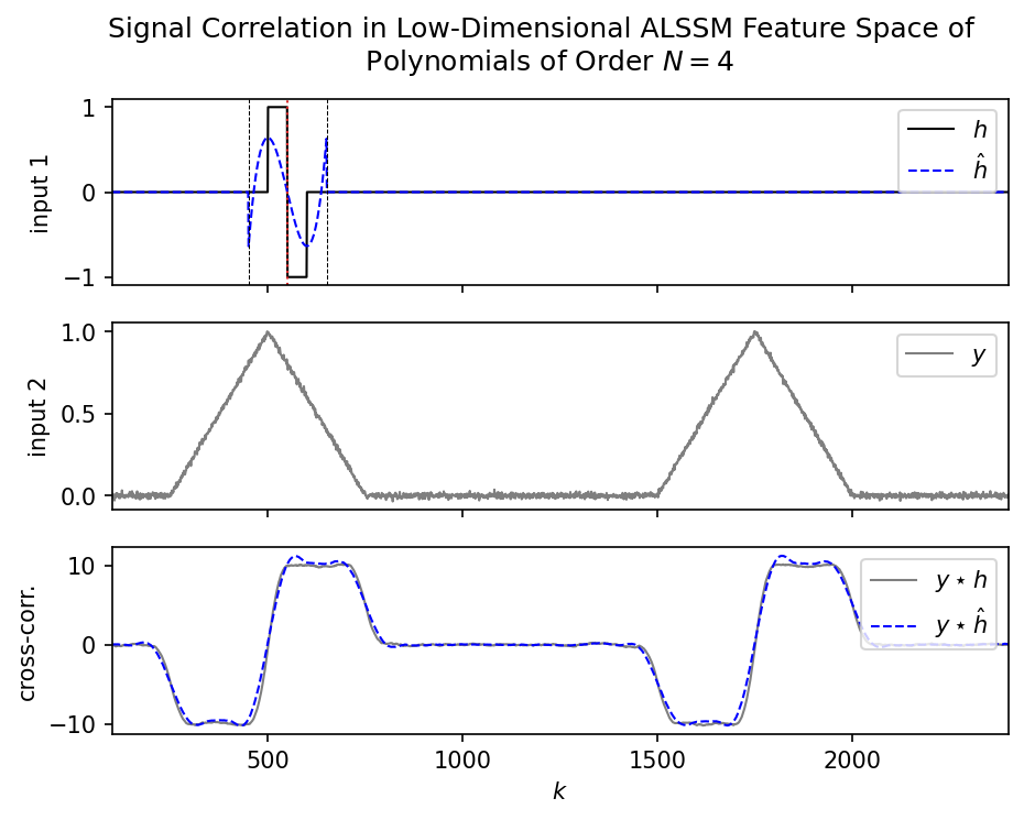
Cross-correlates a noisy sawtooth signal (gray) with a pulse template (black) in a low-dimensional ALSSM feature space.

Both the multi-channel signal and the reference template are projected onto a polynomial basis through an AlssmPolyJordan model. The template's state vector is extracted and correlated against the signal with RLSAlssm.convolve, and the output is compared against the direct sample-domain cross-correlation.

Plot

Console Output

/home/runner/work/lmlib/lmlib/examples/50-convolution/_temp_example-ex504.0-correlation_triangle.py:67: FutureWarning: create_rls() is deprecated and will be removed in a future version. Instantiate RLSAlssm object directly with e.g. rls = lm.RLSAlssm(cost)
  rls_y = lm.create_rls(cost, multi_channel_set=True)
/home/runner/work/lmlib/lmlib/examples/50-convolution/_temp_example-ex504.0-correlation_triangle.py:72: FutureWarning: create_rls() is deprecated and will be removed in a future version. Instantiate RLSAlssm object directly with e.g. rls = lm.RLSAlssm(cost)
  rls_h = lm.create_rls(cost, multi_channel_set=True)
/home/runner/work/lmlib/lmlib/examples/50-convolution/_temp_example-ex504.0-correlation_triangle.py:80: UserWarning: convolve() only requires xi; disabling calc_W and calc_kappa for this RLSAlssm. Construct it with calc_W=False, calc_kappa=False to avoid this warning.
  corr_alssm = rls_y.convolve(y_mc, xs_h)

Code

r"""
Correlation with a Triangular Pulse Template in Low-Dimensional ALSSM
Feature Space [ex504.0]
======================================================================

Cross-correlates a noisy sawtooth signal (gray) with a pulse
template (black) in a low-dimensional ALSSM feature space.

Both the multi-channel signal and the reference template are projected onto
a polynomial basis through an [`AlssmPolyJordan`][lmlib.statespace.model.AlssmPolyJordan]
model. The template's state vector is extracted and correlated against the signal with
[`RLSAlssm.convolve`][lmlib.statespace.rls.RLSAlssm.convolve],
and the output is compared against the direct sample-domain cross-correlation.
"""
import numpy as np
import matplotlib.pyplot as plt

import lmlib as lm
from lmlib.utils.generator import gen_wgn

# -- 0. Generate Test signal ---
K = 2500  # number of samples to process
k = range(K)
ka = np.array(k)

NOFCH = 1  # number of channels
K_REF = 550  # Location of reference template (Index of shape to correlate with)
H_PULSE_WIDTH_2 = 50  # half-width of the triangular template

# Noisy sawtooth signal y: two ramps (rising/falling) repeating every 5 periods of 250 samples
saw_signal_rising = np.mod(ka / 250, 1)
saw_signal_rising[np.mod(ka // 250, 5) != 1] = 0

saw_signal_falling = 1 - np.mod(ka / 250, 1)
saw_signal_falling[np.mod(ka // 250, 5) != 2] = 0

saw_signal = saw_signal_rising + saw_signal_falling
y_mc = np.outer(saw_signal + gen_wgn(K, .010, seed=156789), np.ones([NOFCH]))  # Generate Test signal.

# Triangular pulse template h, centered at K_REF: rising edge then falling edge
h_mc = -np.outer(np.ones(K), np.ones([NOFCH]))
h_mc[:K_REF - H_PULSE_WIDTH_2, :] = 0
h_mc[K_REF - H_PULSE_WIDTH_2:K_REF, :] = 1
h_mc[K_REF:K_REF + H_PULSE_WIDTH_2, :] = -1
h_mc[K_REF + H_PULSE_WIDTH_2:, :] = 0

# -- 1. Polynomial ALSSM model for later signal approximation --
a = -100  # length of shape to correlate with, i.e., uses samples {K_REF+a, ..., K_REF+b} as the correlation template
b = 100
N = 4  # polynomial order (number of coefficients)
alssm = lm.AlssmPolyJordan(poly_degree=N, label='Alssm')
segment = lm.Segment(a=a, b=b, direction=lm.BACKWARD, g=3800)
cost = lm.CostSegment(alssm, segment)

# -- 2. Project observation y to ALSSM feature space --
rls_y = lm.create_rls(cost, multi_channel_set=True)
rls_y.filter(y_mc)  # Transform observations
xs_hat = rls_y.minimize_x()  # get transformed observations

# -- 3. Project template h to ALSSM feature space --
rls_h = lm.create_rls(cost, multi_channel_set=True)
rls_h.filter(h_mc)  # Transform observations
xs_h_hat = rls_h.minimize_x()  # get transformed observations
xs_h = xs_h_hat[K_REF, :]  # get correlation template

y_hat = cost.eval_alssm_output(xs_hat)  # signal reconstruction using ALSSM approximation (for illustration only)

# -- 4. Fast correlation in ALSSM feature space (channel-wise) --
corr_alssm = rls_y.convolve(y_mc, xs_h)

# -- 5. Standard correlation in sample space (channel-wise) (for comparison) --
corr_native = np.zeros(y_mc.shape[0])
h_mc_seg = h_mc[K_REF + a:K_REF + b + 1, :]  # cut out template segment
for j in range(NOFCH):
    corr_native[-a:-a + K - (b - a)] += np.correlate(y_mc[:, j], h_mc_seg[:, j], 'valid')

# -- 6. Plotting --
template_trajectory = lm.Trajectory.eval_y(cost, xs_h, K_REF, K, fill_value=0.0)

_, axs = plt.subplots(3, 1, figsize=(7, 5), gridspec_kw={'height_ratios': [1, 1, 1]}, sharex='all')
nax = 0
offsets = (np.arange(NOFCH, 0, -1) - 1) * .5

# Template h
axs[nax].plot(k, h_mc + offsets, c='k', lw=1.0, label=['$h$'])
axs[nax].plot(k, template_trajectory + offsets, '--', c='blue', lw=1.0, label=[r'$\hat h$'])
axs[nax].axvline(K_REF + a, color="black", linestyle="--", lw=0.5)
axs[nax].axvline(K_REF + b, color="black", linestyle="--", lw=0.5)
axs[nax].axvline(K_REF, color="tab:red", linestyle=":", lw=1.0)
axs[nax].legend(loc='upper right')
axs[nax].set(ylabel='input 1')

# Observation y
nax += 1
axs[nax].plot(k, y_mc + offsets, c='tab:gray', lw=1, label=['$y$'])
axs[nax].legend(loc='upper right')
axs[nax].set(ylabel='input 2')

# Correlation
nax += 1
axs[nax].set(xlabel='$k$')
axs[nax].plot(k, corr_native, c='tab:gray', lw=1, linestyle='-', label=r"$y \star h$")
axs[nax].plot(k, corr_alssm, '--', c='b', lw=1, label=r"$y \star \hat h$")
axs[nax].legend(loc='upper right')
axs[nax].set(ylabel='cross-corr.')
axs[nax].set_xlim(100, K - 100)

plt.suptitle(f"Signal Correlation in Low-Dimensional ALSSM Feature Space of \n Polynomials of Order $N={N}$")
plt.show()