Audio Signal Shift Estimation [ex702.0]
Example 2 as published in [Wildhaber2020].
Equation references in the code (e.g. # Eq. 6.52) refer to equations
in [Wildhaber2019].
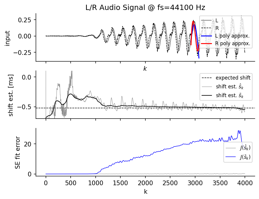
Top plot: Two-channel acoustic signal from the left (L) and right (R) ear with an unknown interaural time delay (ITD) to be estimated.
Middle plot: Local time-delay estimates from corresponding local polynomial fits (per-sample estimate and running average).
Bottom plot: Estimated delay overlaid on the signal.
The shift is estimated by comparing the polynomial coefficients of the two channels within a sliding window, exploiting the algebraic shift relationship between the polynomial bases of the left and right channels.
Plot
Data
This example uses the following data file(s):
Code
r"""
Audio Signal Shift Estimation [ex702.0]
=======================================
Example 2 as published in [\[Wildhaber2020\]](../../../bibliography.md#wildhaber2020).
Equation references in the code (e.g. ``# Eq. 6.52``) refer to equations
in [\[Wildhaber2019\]](../../../bibliography.md#wildhaber2019).

**Top plot:** Two-channel acoustic signal from the left (L) and right (R)
ear with an unknown interaural time delay (ITD) to be estimated.

**Middle plot:** Local time-delay estimates from corresponding local
polynomial fits (per-sample estimate and running average).

**Bottom plot:** Estimated delay overlaid on the signal.

The shift is estimated by comparing the polynomial coefficients of the two
channels within a sliding window, exploiting the algebraic shift relationship
between the polynomial bases of the left and right channels.
"""

import numpy as np
import matplotlib.pyplot as plt
import os

import lmlib as lm
from lmlib.utils import load_csv_mc


def const_shift_estimations(Q, a, b):
    # the multiplication on the A, B, C matrices creates numerical issues , so in this from it's not applicable for high order systems
    # assert False
    q = np.arange(Q)
    L_shift = lm.mpoly_shift_coef_L(q)  # Eq. 6.52
    q_shift, _ = lm.mpoly_shift_expos(q)  # Eq, 6.51
    Lt = np.diag(np.kron(1 ** q_shift, (-0.5) ** q_shift)) @ L_shift  # Eq. 6.54
    Bt = np.diag(np.kron(1 ** q_shift, 0.5 ** q_shift)) @ L_shift  # Eq. 6.54

    R = lm.mpoly_square_coef_L((q_shift, q_shift))  # Eq. 6.103
    qp, _ = lm.mpoly_square_expos((q_shift, q_shift))
    L_def_int = lm.mpoly_def_int_coef_L((qp, qp), 0, a, b)  # Eq. 6.61, Eq. 6.62
    Ct = L_def_int @ R  #
    Kt = np.eye(Bt.shape[1] ** 4) + lm.permutation_matrix_square(Bt.shape[1], Lt.shape[1])  # Eq. 6.115
    A = Ct @ np.kron(Lt, Lt)
    B = Ct @ Kt @ np.kron(Lt, Bt)
    C = Ct @ np.kron(Bt, Bt)
    return A, B, C, qp


def const_shift_estimations2(Q, a, b):
    q = np.arange(Q)
    L_shift = lm.mpoly_shift_coef_L(q)  # Eq. 6.52
    q_shift, _ = lm.mpoly_shift_expos(q)  # Eq, 6.51
    Lt = np.diag(np.kron(1 ** q_shift, (-0.5) ** q_shift)) @ L_shift  # Eq. 6.54
    Bt = np.diag(np.kron(1 ** q_shift, 0.5 ** q_shift)) @ L_shift  # Eq. 6.54

    R = lm.mpoly_square_coef_L((q_shift, q_shift))  # Eq. 6.103
    qp, _ = lm.mpoly_square_expos((q_shift, q_shift))
    L_def_int = lm.mpoly_def_int_coef_L((qp, qp), 0, a, b)  # Eq. 6.61, Eq. 6.62
    Ct = L_def_int @ R  #
    Kt = np.eye(Bt.shape[1] ** 4) + lm.permutation_matrix_square(Bt.shape[1], Lt.shape[1])  # Eq. 6.115
    A = Ct @ np.kron(Lt, Lt)
    B = Ct @ Kt @ np.kron(Lt, Bt)
    C = Ct @ np.kron(Bt, Bt)
    return Lt, Bt, Ct, qp


def poly_newton(alphaD, qD, alphaDD, qDD, x0, min_step):
    cur_x = np.array(x0).astype('float').copy()
    step = float('inf')
    iter = 0
    while step >= min_step and iter < 100:
        iter += 1
        prev_x = cur_x.copy()
        delta_x = (alphaD.T @ (prev_x ** qD)) / (alphaDD.T @ (prev_x ** qDD))
        step = (alphaD.T @ prev_x ** qD) * delta_x
        cur_x = prev_x - delta_x
    return cur_x


try:
    SCRIPT_DIR = os.path.dirname(os.path.abspath(__file__))
except NameError:
    SCRIPT_DIR = os.getcwd()
csv_file = os.path.join(SCRIPT_DIR, "shift_estimation_data.csv")
y = load_csv_mc(csv_file)
true_shift = .52e-3  # seconds
fs = 44100
K = len(y)
t = np.arange(K) / fs

method_py_stable = True  # numerical stable

# setup polynomial model and filer signal
alssm = lm.AlssmPoly(poly_degree=3)
segment_left = lm.Segment(a=-80, b=-1, direction=lm.FW, g=600)
segment_right = lm.Segment(a=0, b=80 - 1, direction=lm.BW, g=600)
cost = lm.CompositeCost([alssm], [segment_left, segment_right], F=[[1, 1]])
rls = lm.RLSAlssm(cost)
rls.filter(y)
xs = rls.minimize_x()

# boundaries cost function
a = segment_left.a * 0.8
b = segment_right.b * 0.8

# get polynomial cost function matrices
A, B, C, _ = const_shift_estimations(alssm.N, a, b)  # if method_py_stable == True
Lt, Bt, Ct, q = const_shift_estimations2(alssm.N, a, b)  # if method_py_stable == True

# get derivative matrices for optimization
Ld = lm.poly_diff_coef_L(q)
qd = lm.poly_diff_expo(q)
Ldd = lm.poly_diff_coef_L(qd) @ Ld
qdd = lm.poly_diff_expo(qd)

# moving averaged shift range
k_span = np.arange(-100, 101, 1)

# -------- shift estimation ------------
Js = np.full(K, np.nan)
shifts_hat = np.zeros(K)

for k0 in range(K):
    alpha = xs[k0, 0]
    beta = xs[k0, 1]

    if method_py_stable:
        alphas = (Ct @ np.kron(Lt @ alpha - Bt @ beta, Lt @ alpha - Bt @ beta))
    else:
        alphas = (A @ np.kron(alpha, alpha) - B @ np.kron(alpha, beta) + C @ np.kron(beta, beta))

    shifts_hat[k0] = poly_newton(Ld @ alphas, qd, Ldd @ alphas, qdd, shifts_hat[k0 - 1], min_step=1e-12)
    Js[k0] = alphas.T @ shifts_hat[k0] ** q

# -------- smooth moving averaged estimation of the shift ------------
shifts_hat_MA = np.zeros(K)
Js_MA = np.full(K, np.nan)

for k0 in range(K):

    alphas = np.zeros(Ct.shape[0])

    for k in np.unique(np.clip(k_span + k0, 0, K - 1)):
        alpha = xs[k, 0]
        beta = xs[k, 1]
        if method_py_stable:
            alphas += (Ct @ np.kron(Lt @ alpha - Bt @ beta, Lt @ alpha - Bt @ beta))
        else:
            alphas += (A @ np.kron(alpha, alpha) - B @ np.kron(alpha, beta) + C @ np.kron(beta, beta))
        shifts_hat_MA[k0] = poly_newton(Ld @ alphas, qd, Ldd @ alphas, qdd, shifts_hat_MA[k0 - 1], min_step=1e-12)
        Js_MA[k0] = alphas.T @ shifts_hat_MA[k0] ** q

# -------- plot ------------

ks = [2997]  # index of trajectories
trajs = lm.Trajectory.eval_y(cost, xs[ks], ks, K)

fig, axs = plt.subplots(3, sharex='all')
axs[0].plot(y[:, 0], '-', c=(0.3,) * 3, lw=.8, label='L')
axs[0].plot(y[:, 1], '--', c=(0,) * 3, lw=.8, label='R')
axs[0].plot(trajs[:, 0], c='b', label='L poly approx.')
axs[0].plot(trajs[:, 1], c='r', label='R poly approx.')
axs[0].legend(loc=1, fontsize=8)
axs[0].set(ylabel='input', xlabel='$k$')
axs[0].set_title(f'L/R Audio Signal @ fs={fs} Hz')

if False:  # plotting of shift-corrected signals
    print(np.median(shifts_hat), np.median(shifts_hat) / fs)
    k_corr_ch1 = np.clip(np.arange(K) - int(np.median(shifts_hat) / 2), 0, K - 1)
    k_corr_ch2 = np.clip(np.arange(K) + int(np.median(shifts_hat) / 2), 0, K - 1)
    axs[0].plot(y[k_corr_ch1, 0], c='b', ls='--', lw=1, label='# 1')
    axs[0].plot(y[k_corr_ch2, 1], c='r', ls='--', lw=1, label='# 2')
    axs[0].legend(loc=1, fontsize=8)

axs[1].axhline(-true_shift * 1000, c='k', ls='--', lw=0.8, label='expected shift')
axs[1].plot(shifts_hat / fs * 1000, c='gray', lw=0.5, label=r'shift est. $\hat{s}_k$')
axs[1].plot(shifts_hat_MA / fs * 1000, c='k', lw=1.0, label=r'shift est. $\bar{s}_k$')
axs[1].legend(loc=1, fontsize=8)
axs[1].set(ylabel='shift est. [ms]')
axs[1].set_ylim(-0.7, 0.1)

axs[2].plot(Js, c='gray', lw=0.5, label=r'$J(\hat{s}_k)$')
axs[2].plot(Js_MA, c='blue', lw=0.75, label=r'$J(\bar{s}_k)$')
axs[2].legend(loc='center right', fontsize=8)
axs[2].set_xlabel('k')
axs[2].set(ylabel='SE fit error')

for _ax in axs:
    _ax.spines['top'].set_visible(False)
    _ax.spines['right'].set_visible(False)

plt.show()