Time and Amplitude Scaling [ex703.0]

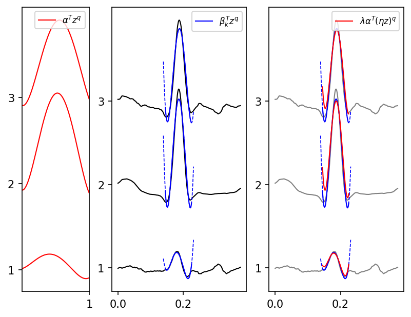
Estimates both a time-scaling (dilation) factor and an amplitude-scaling factor between two locally polynomial signals. This example is published in [Wildhaber2020].

The polynomial coefficients of the reference and the candidate windows are related by the dilation and amplitude operators, enabling a closed-form least-squares estimator via the polynomial calculus.

Plot

Code

r"""
Time and Amplitude Scaling [ex703.0]
====================================

Estimates both a time-scaling (dilation) factor and an amplitude-scaling
factor between two locally polynomial signals.
This example is published in [\[Wildhaber2020\]](../../../bibliography.md#wildhaber2020).

The polynomial coefficients of the reference and the candidate windows are
related by the dilation and amplitude operators, enabling a closed-form
least-squares estimator via the polynomial calculus.
"""

import matplotlib.pyplot as plt
from matplotlib.lines import Line2D

import numpy as np
import lmlib as lm
from lmlib.utils import load_lib_csv_mc


def time_amplitude_scaling(Q, a, b):
    q = np.arange(Q)
    Mq = lm.poly_square_expo(q)
    Mqp1 = lm.poly_int_expo(Mq)
    L_int = lm.poly_int_coef_L(Mq)
    L_eta = lm.mpoly_dilate_ind_coef_L(q)  # matrix operation of vdiag
    R_QQ = lm.permutation_matrix_square(Q, Q)

    I_Q = np.eye(Q)
    I_QQ = np.eye(Q ** 2)

    c1 = L_int
    c2 = np.kron(I_Q, L_int).dot(np.kron(L_eta, I_Q))
    c3 = np.kron(I_QQ, L_int).dot(R_QQ).dot(np.kron(L_eta, L_eta))

    bmaT = (np.power(b, Mqp1) - np.power(a, Mqp1)).T
    A = bmaT @ c1
    B = np.kron(I_Q, bmaT) @ c2
    C = np.kron(I_QQ, bmaT) @ c3

    return A, B, C, q, Mq


y = load_lib_csv_mc('SECG3_FILT_HP51_3CH_20S_FS2400HZ.csv', k_start=5500, K=750)
y = np.column_stack([np.convolve(y0, 1 / 50 * np.ones(50), 'same') for y0 in y.T])

fs = 2000
K = len(y)
t = np.arange(K) / fs
M = 3
Q = 5
ENERGY_THD = 60

ab_half = int((80e-3 * fs) / 2)
ks_alpha = np.array([370])  # fixing template

alssm = lm.AlssmPoly(poly_degree=Q - 1)
segment_right = lm.Segment(a=-ab_half, b=ab_half, direction=lm.BW, g=50, delta=ab_half)
cost = lm.CostSegment(alssm, segment_right)
rls = lm.RLSAlssm(cost)
rls.filter(y)
xs = rls.minimize_x(solver='inv')

# generate template
dilate_factor = 1.456
amplitude_factor = 0.945
y_template = amplitude_factor * np.column_stack(
    [np.interp(np.linspace(0, K, int(K * dilate_factor)), np.arange(K), y0) for y0 in y.T])

rls_tmpl = lm.RLSAlssm(cost)
rls_tmpl.filter(y_template)
xs_tmpl = rls_tmpl.minimize_x(solver='inv')
alphas = xs_tmpl[(ks_alpha * dilate_factor).astype(int)]

A, B, C, q, Mq = time_amplitude_scaling(Q, a=-ab_half, b=ab_half)
etas = np.linspace(0.5, 2, 1000)

J = np.full(K, np.inf)
cost_ratio = np.full(K, np.inf)
model_energy_obs = np.full(K, np.inf)
time_scaling_hat = np.full(K, np.nan)
amplitude_hat = np.full(K, np.nan)

for k in range(K):

    beta_beta = np.zeros(Q ** 2)
    alpha_beta = np.zeros(Q ** 2)
    alpha_alpha = np.zeros(Q ** 2)

    for m in range(M):
        beta_beta += np.kron(xs[k, m], xs[k, m])
        alpha_beta += np.kron(alphas[0, m], xs[k, m])
        alpha_alpha += np.kron(alphas[0, m], alphas[0, m])

    a1 = A @ beta_beta
    for eta in etas:
        J_ = a1 - (((B @ alpha_beta).T @ np.power(eta, q)) ** 2) / ((C @ alpha_alpha).T @ np.power(eta, Mq))
        if J_ < J[k]:
            J[k] = J_
            time_scaling_hat[k] = eta
            amplitude_hat[k] = ((B @ alpha_beta).T @ np.power(eta, q)) / ((C @ alpha_alpha).T @ np.power(eta, Mq))
            cost_ratio[k] = J_ / a1
            model_energy_obs[k] = a1

mask = ENERGY_THD < model_energy_obs
k_range_mask = np.flatnonzero(mask)
k_min = k_range_mask[np.argmin(cost_ratio[mask])]

L_dilate = lm.poly_dilation_coef_L(np.arange(Q), time_scaling_hat[k_min])
alphas_hat = amplitude_hat[k_min] * np.einsum('mn, ksn->ksm', L_dilate, alphas)

# -- Plotting --


# Plot A: Trajectories
offset_channels = np.arange(M) + 1
fig, (ax1, ax2, ax3) = plt.subplots(1, 3, gridspec_kw={'width_ratios': [1, 2, 2]})
ab_half_ext = int(ab_half * 1.15)
segment_right = lm.Segment(a=-ab_half_ext, b=ab_half_ext, direction=lm.BW, g=50, delta=ab_half_ext)
cost_ext = lm.CostSegment(alssm, segment_right)

trajs_obs      = lm.Trajectory.eval_y(cost, xs[ks_alpha], ks_alpha, K)
trajs_tmpl_hat = lm.Trajectory.eval_y(cost, alphas_hat, k_min, K)
trajs_obs_ext  = lm.Trajectory.eval_y(cost_ext, xs[ks_alpha], ks_alpha, K)

k_tmpl, trajs_tmpl = zip(*lm.Trajectory.eval(cost, alphas, merged_ks=True,merged_seg=True))
k_tmpl = np.array(k_tmpl[0])   # all ranges identical, take first
trajs_tmpl = np.array(trajs_tmpl).T #have K in first dimension

ax1.plot(k_tmpl, trajs_tmpl + offset_channels, lw=1, c='r', label=r'$\alpha^T z^q$')

ax1.set_xlim([min(k_tmpl), max(k_tmpl)])
ax1.set_xticks([max(k_tmpl)])
ax1.set_xticklabels(['1'])
ax1.legend([Line2D([0], [0], color='r', lw=1)], [r'$\alpha^T z^q$'], loc=1, fontsize=8)

ax2.plot(t, y + offset_channels, lw=1, c='k')
ax2.plot(t, trajs_obs_ext +  offset_channels, lw=0.8, ls='--', c='b')
ax2.plot(t, trajs_obs +  offset_channels, lw=1, c='b')
ax2.legend([Line2D([0], [0], color='b', lw=1)], [r'$\beta_k^T z^q$'], loc=1, fontsize=8)

ax3.plot(t, y + offset_channels, lw=1, c='grey')
ax3.plot(t, trajs_obs_ext + offset_channels, lw=0.8, ls='--', c='b')
ax3.plot(t, trajs_obs  + offset_channels, lw=1, c='b')
ax3.plot(t, trajs_tmpl_hat  + offset_channels, lw=1, c='r', label=r'$\alpha^T z^q$')
ax3.legend([Line2D([0], [0], color='r', lw=1)], [r'$\lambda \alpha^T (\eta z)^q$'], loc=1, fontsize=8)

for ax in fig.axes:
    ax.set_yticks([1, 2, 3])

plt.show()

# Plot B: Show cost and estimate over time
if True:
    fig, axs = plt.subplots(5, 1, sharex='all')
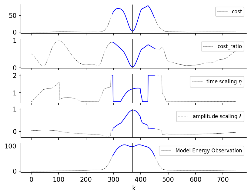
    axs[0].plot(J, c='k', lw=0.6, ls=':', label='cost')
    axs[0].plot(k_range_mask, J[mask], c='b', lw=1)
    axs[1].plot(cost_ratio, c='k', lw=0.6, ls=':', label='cost_ratio')
    axs[1].plot(k_range_mask, cost_ratio[mask], c='b', lw=1)
    axs[2].plot(time_scaling_hat, c='k', lw=0.6, ls=':', label=r'time scaling $\eta$')
    axs[2].plot(k_range_mask, time_scaling_hat[mask], c='b', lw=1)
    axs[3].plot(amplitude_hat, c='k', lw=0.6, ls=':', label=r'amplitude scaling $\lambda$')
    axs[3].plot(k_range_mask, amplitude_hat[mask], c='b', lw=1)
    axs[4].plot(model_energy_obs, c='k', lw=0.6, ls=':', label=r'Model Energy Observation')
    axs[4].plot(k_range_mask, model_energy_obs[mask], c='b', lw=1)
    for ax in axs:
        ax.axvline(k_min, c='k', lw=0.5)
        ax.legend(loc=1, fontsize=8)
        ax.spines['top'].set_visible(False)
        ax.spines['right'].set_visible(False)
    axs[-1].set_xlabel('k')
    plt.show()