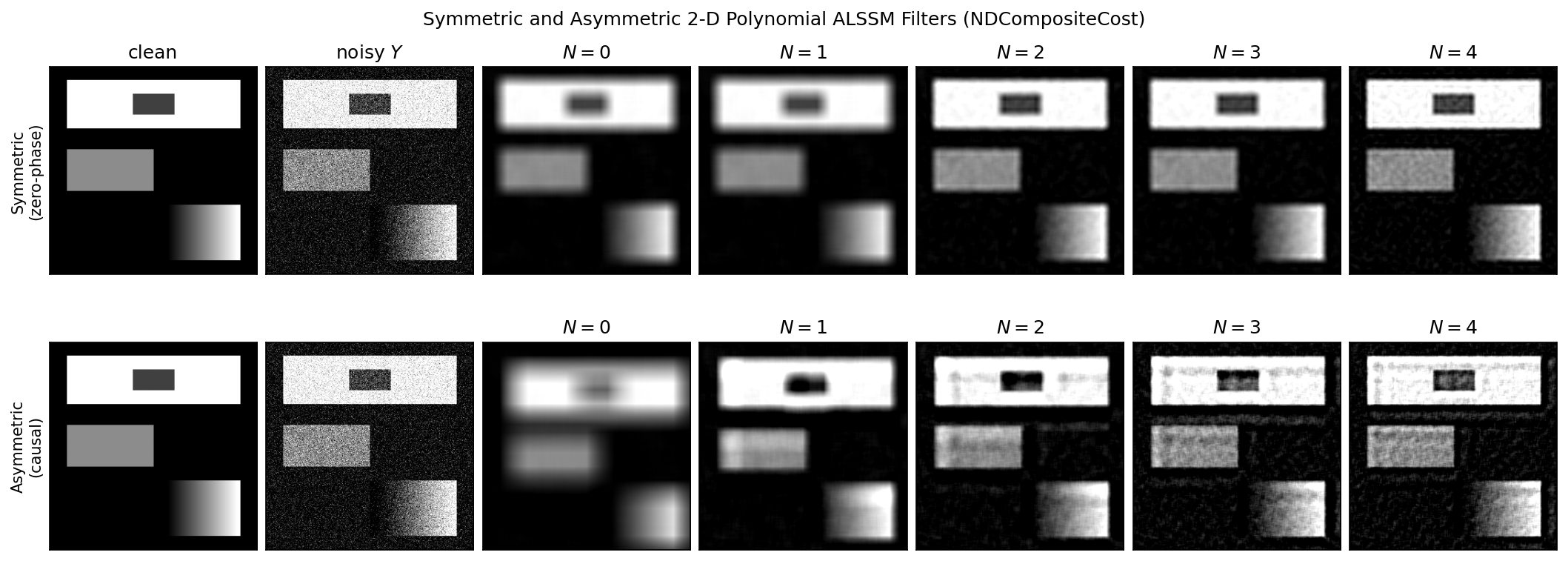
Symmetric and Non-Symmetric 2-D Polynomial Filters with ALSSMs [ex126.0]
2-D extension of the 1-D polynomial smoother shown in ex122.0.
Instead of a single CompositeCost,
a separable NDCompositeCost is built
from one polynomial CompositeCost per
image axis and applied to a noisy 2-D signal (an image) in a single
fit call. At every pixel the filter fits a
separable polynomial surface of degree N to the surrounding window and
returns the surface value at the window centre.
Two filter configurations are shown for each polynomial degree:
- Symmetric filter — forward (left/top) and backward (right/bottom)
windows of equal size on every axis (mixing matrix
F = [[1, 1]]), yielding a zero-phase (non-causal) 2-D smoother. - Asymmetric filter — a single forward window from the left/top
side of every axis (mixing matrix
F = [[1]]).
Higher polynomial degrees follow the image edges more closely but are more sensitive to noise in flat regions.
Plot
Code
"""
Symmetric and Non-Symmetric 2-D Polynomial Filters with ALSSMs [ex126.0]
========================================================================

2-D extension of the 1-D polynomial smoother shown in
[ex122.0](../12-filtering/example-ex122.0-polynomial-filters-pascal.md).

Instead of a single [`CompositeCost`][lmlib.statespace.cost.CompositeCost],
a separable [`NDCompositeCost`][lmlib.statespace.cost.NDCompositeCost] is built
from one polynomial [`CompositeCost`][lmlib.statespace.cost.CompositeCost] **per
image axis** and applied to a noisy 2-D signal (an image) in a single
[`fit`][lmlib.statespace.rls.RLSAlssm.fit] call. At every pixel the filter fits a
separable polynomial surface of degree ``N`` to the surrounding window and
returns the surface value at the window centre.

Two filter configurations are shown for each polynomial degree:

* **Symmetric filter** — forward (left/top) *and* backward (right/bottom)
  windows of equal size on every axis (mixing matrix ``F = [[1, 1]]``),
  yielding a zero-phase (non-causal) 2-D smoother.
* **Asymmetric filter** — a single forward window from the left/top
  side of every axis (mixing matrix ``F = [[1]]``).

Higher polynomial degrees follow the image edges more closely but are more
sensitive to noise in flat regions.
"""

import matplotlib.pyplot as plt
import numpy as np
import lmlib as lm
from lmlib.utils.generator import gen_wgn
plt.close('all')

# --- Generating a 2-D test signal (image) -----------------------------------
# A piecewise-constant image with sharp edges (the 2-D analogue of the
# rectangular test signal `gen_rect` used in ex122) plus a diagonal intensity
# ramp, contaminated with white Gaussian noise.
K1, K2 = 300, 300                       # image size (rows, cols)
img = np.zeros((K1, K2))
img[20:90, 25:275] = 1.00               # bright block
img[40:70, 120:180] = 0.25              # dark inset inside the bright block
img[120:180, 25:150] = 0.55             # mid-gray block
rr, cc = np.mgrid[0:K1, 0:K2]           # diagonal ramp region (tests poly degree)
img[200:280, 150:275] = 0.30 + 0.5 * (cc[200:280, 150:275] - 200) / 50

Y = img + gen_wgn((K1, K2), 0.18, seed=1)   # noisy observation

# --- Filter configuration ----------------------------------------------------
DEGREES = (0, 1, 2, 3, 4)                  # polynomial degrees, as in ex122
L = 10                                     # half-window length (samples per side)
G = 40                                     # effective window weight (samples)


def make_nd_cost(poly_degree, symmetric):
    """Build a separable 2-D polynomial NDCompositeCost.

    One identical 1-D polynomial CompositeCost is used on each image axis.

    Parameters
    ----------
    poly_degree : int
        Degree of the per-axis polynomial ALSSM.
    symmetric : bool
        If True, use forward + backward windows (``F = [[1, 1]]``,
        zero-phase). If False, use the forward window only
        (``F = [[1]]``, causal / phase-delayed).
    """
    #alssm_poly = lm.AlssmPolyJordan(poly_degree=poly_degree)
    alssm_poly = lm.AlssmPolyLegendre(poly_degree=poly_degree,a_seg=-L, b_seg=L)

    # one CompositeCost per image dimension, wrapped into an NDCompositeCost
    if symmetric:
        segment_left = lm.Segment(a=-L, b=0, direction=lm.FORWARD, g=G)
        segment_right = lm.Segment(a=1, b=L, direction=lm.BACKWARD, g=G)
        F = [[1, 1]]
        cost_dim1 = lm.CompositeCost((alssm_poly,), (segment_left, segment_right), F=F)
        cost_dim2 = lm.CompositeCost((alssm_poly,), (segment_left, segment_right), F=F)
    else:
        #segment_left = lm.Segment(a=-L//2, b=L//2, direction=lm.FORWARD, g=G)
        segment_left = lm.Segment(a=-L*4, b=0, direction=lm.FORWARD, g=G)
        F = [[1]]
        cost_dim1 = lm.CompositeCost((alssm_poly,), (segment_left, ), F=F)
        cost_dim2 = lm.CompositeCost((alssm_poly,), (segment_left, ), F=F)
    return lm.NDCompositeCost([cost_dim1, cost_dim2])


# --- 2-D ALSSM filtering -----------------------------------------------------
y_hats_sym = []     # symmetric (zero-phase) results, one per degree
y_hats_asym = []    # asymmetric (causal) results, one per degree

for degree in DEGREES:
    # -- Symmetric Filter --
    nd_cost = make_nd_cost(degree, symmetric=True)
    rls = lm.RLSAlssm(nd_cost, steady_state=True, backend='lfilter')
    y_hats_sym.append(rls.fit(Y))

    # -- Asymmetric (causal) Filter --
    nd_cost = make_nd_cost(degree, symmetric=False)
    rls = lm.RLSAlssm(nd_cost, steady_state=True, backend='lfilter')
    y_hats_asym.append(rls.fit(Y))

# --- Plotting ----------------------------------------------------------------
imshow_kw = dict(cmap='gray', vmin=0.0, vmax=1.0)
n_cols = len(DEGREES) + 2                 # clean + noisy + one column per degree
fig, ax = plt.subplots(2, n_cols, figsize=(2.0 * n_cols, 5.2),
                       constrained_layout=True)

for row in range(2):
    ax[row, 0].imshow(img, **imshow_kw)
    ax[row, 0].set_ylabel('Symmetric\n(zero-phase)' if row == 0
                          else 'Asymmetric\n(causal)', fontsize=10)
    ax[row, 1].imshow(Y, **imshow_kw)

ax[0, 0].set_title('clean')
ax[0, 1].set_title('noisy $Y$')

for col, degree in enumerate(DEGREES, start=2):
    ax[0, col].imshow(y_hats_sym[col - 2], **imshow_kw)
    ax[0, col].set_title(rf'$N={degree}$')
    ax[1, col].imshow(y_hats_asym[col - 2], **imshow_kw)
    ax[1, col].set_title(rf'$N={degree}$')

for a in ax.flat:
    a.set_xticks([])
    a.set_yticks([])

fig.suptitle('Symmetric and Asymmetric 2-D Polynomial ALSSM Filters '
             '(NDCompositeCost)', fontsize=12)
plt.show()